Mask and Parameters

General Parameters:

Load Parameters:

Ports, Inputs, Outputs and Signals Available for Monitoring

Ports

• Net_1: Network connection (supports only 1-phase connections)

Inputs

• None

Outputs

• None

Sensors

• F: Estimated current at the point of connection
• Lout: Effective inductance or Capacitance
• Rout: Effective resistance
• Vrms: Estimated RMS voltage at the point of connection

Description of the Load Model

Load Model

The PQ load consists of the series combination of equivalent R, L and C branches and the series combination of equivalent R and L branches. The following rules are applied:

• If P=0 and Q=0, the element becomes disconnected in all solution methods.
• The RL series inductance equivalent is calculated using:

L(Q>0) = {V_{base}^2 \cdot Q \over \omega \cdot (P^2 + Q^2)}

• The resistance value in the RL series combination is given by:

R = {V_{base}^2 \cdot P \over (P^2 + Q^2)}

• When Q<0, the capacitance value becomes:

C(Q<0) = \frac{P^2 + Q^2}{V_{base}^2 \cdot Q  \cdot \omega }

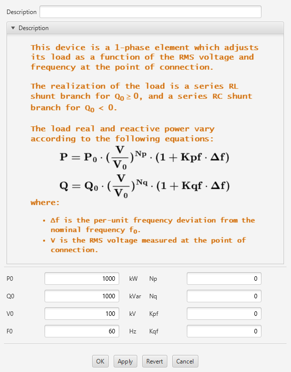
Model Equations

The model equations of this load are given by:

P=P_0\cdot\left(\frac{V}{V_0}\right)^{Np}\cdot(1+Kpf\cdot \Delta f)

Q=Q_0\cdot\left(\frac{V}{V_0}\right)^{Nq}\cdot(1+Kqf\cdot \Delta f)

where:

By adjusting Np and Nq equal to 0, 1, or 2, the load can be set to work as a constant power, constant current, or constant impedance, respectively.