Documentation Home Page ◇ HYPERSIM Home Page
Pour la documentation en FRANÇAIS, utilisez l'outil de traduction de votre navigateur Chrome, Edge ou Safari. Voir un exemple.
Examples | Data Logger
Location
This example model can be found in the software under the category "How To" with the file name "Data_Logger.ecf".
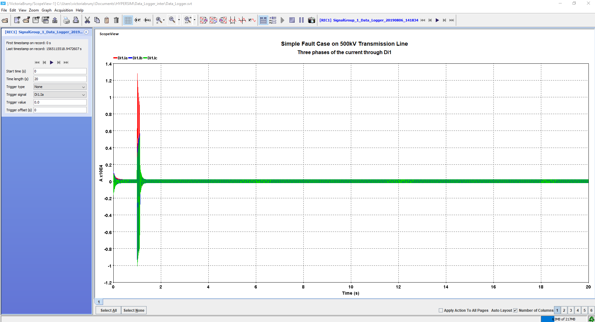
Description
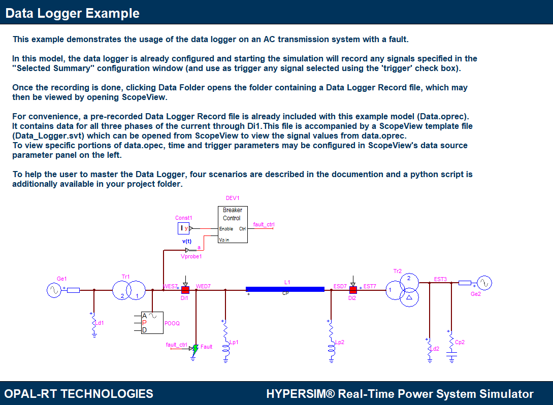
This example demonstrates how some of the data logger features work and how to visualize with ScopeView.
For more details on the configuration, look at HYPERSIM Data Logger.
All the scenarios can run either on the localhost or the real-time simulator.
Note: the Python script is configured to run on localhost, but the code can be modified to make it work in real time on your target using the Target IP address.
Simulation and Results
Sensor Configuration File
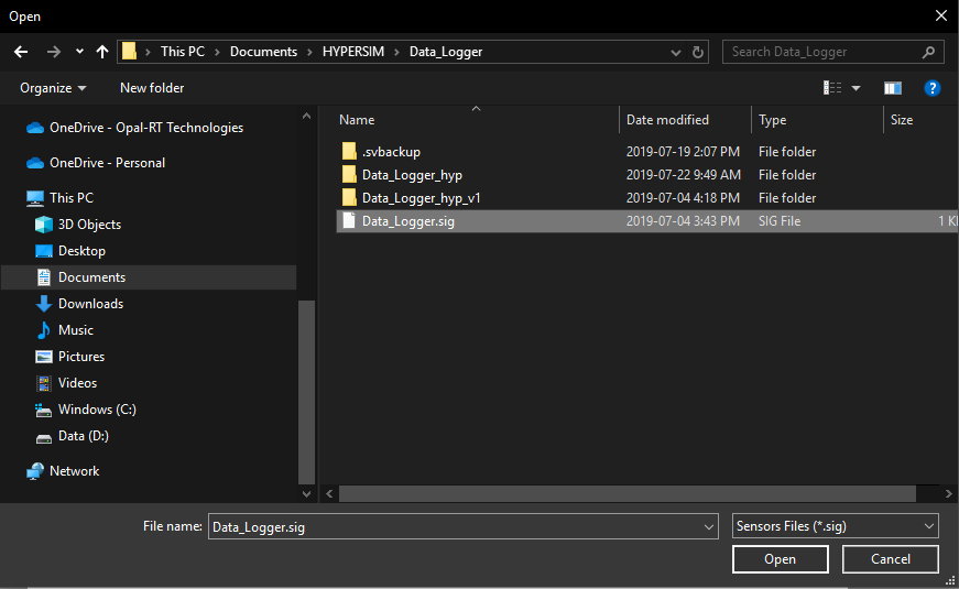
Before running this example, you need to open the sensors file (Data_Logger.sig) included in the example model folder.
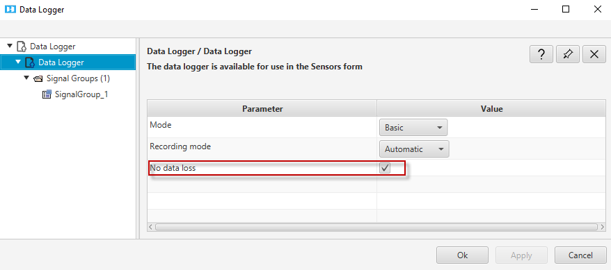
Data Logger Default Settings
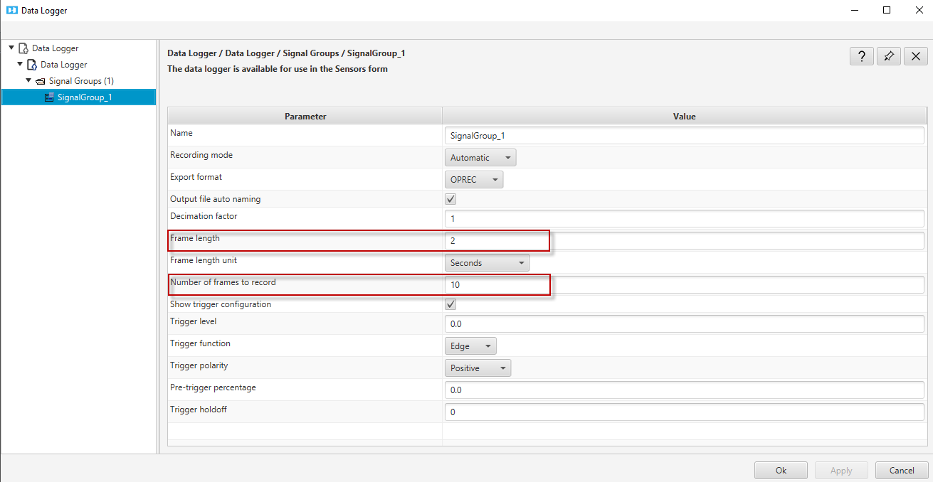
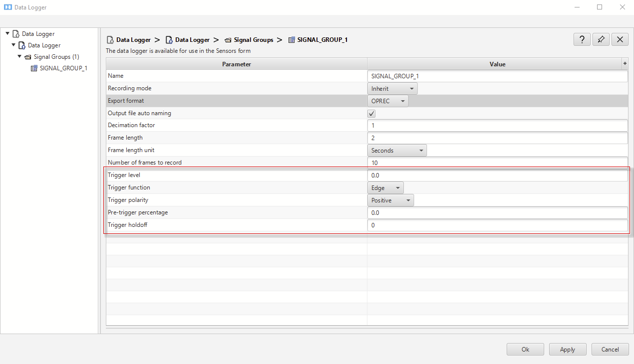
In this following configuration we record 10 frames of 2 seconds each, which means that the data logger is recording a total of 20 seconds of acquisition.
Note: If you run the simulation on localhost, you have to configure the data logger with No data loss.
Recording Mode
In this scenario, we record 10 frames of 2 seconds (see default configuration).
Starting the simulation will record any signals specified in the "Selected Summary" configuration window.
Note: If you don't have any signals in this window you can either open Data_Logger.sig file in Sensors or select your own sensors.
Now, you're ready to start the simulation.
Once the recording is done, clicking on Recording Manager (under Data Logger in the ribbon) will open the folder containing Data Logger Record files.
For better visualization, use the ScopeView template Data_Logger.svt and replace the data source (.oprec recorded in the data folder) by clicking on Data Source then Replace in ScopeView.
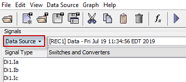
For more information on how to use ScopeView, visit the following link: ScopeView | Main Window
Results
Ensure the Recording Mode is set to Manual (refer to the Data Logger Configuration for details). Manual mode allows you to trigger when you want to record the data.
- In order to proceed, you need to keep the data logger window open and go to Signal Groups (N).
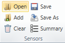
- To start recording, click on the record button
- To stop recording, you can either wait for the 20 seconds of recording to be done (in this example, 10 frames of 2 seconds) or interrupt the record by clicking on the stop recording button.
- Once the recording is done and the simulation is stopped, you can access the data by opening the Recording Manager (under Data Logger in the ribbon).
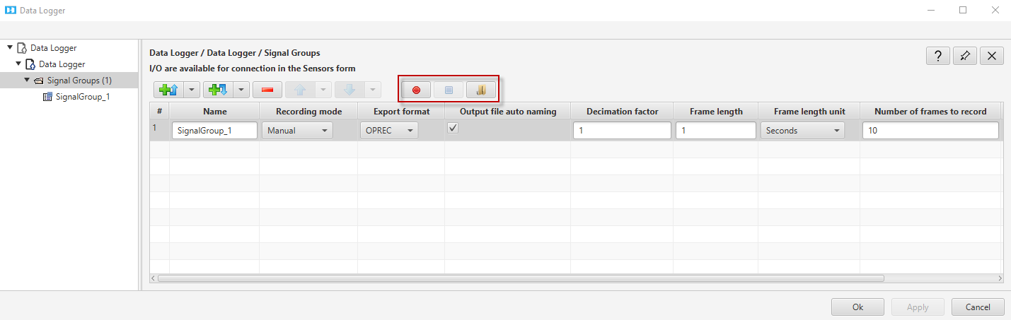
Frames
For each signal group, you can choose the length of record using different units and multiple frames.
You can set up different parameters such as:
- Decimation factor: Number of steps recorded = total number of steps divided by the decimation factor. When set to 1, the samples from each calculation step are stored. When set to 2, the samples from each 2 calculations are stored, etc.
- Frame length: maximum number of samples per frame (unit specified below) to be stored in the data file. Uses the maximum expected file size the data file may reach so that it does not fill the hard drive.
- Frame units: May be either a number of steps, a duration in various time units ranging from nanoseconds to hours, or a file size in megabytes.
- Number of frames to record: number of frame to record. if the frame length is 1 second and we record 10 frames, we will have 10 seconds recorded.
Note: The memory of the data files updates every time a frame is recorded so if you record 100 seconds in 1 frame, you will get the result only after 100 seconds but if you record 1 second and 100 frames, you will be able to look at the waveforms at every second while the data logger is recording.
Example
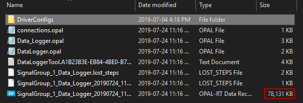
We record 1 second per frame and 100 frames.
As soon as the simulation is started, you can access the IOData sub-folder from code directory and observe that the file size is increasing.
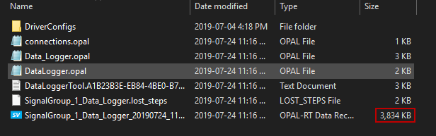
Press F5 to update the refresh the folder and see the updated file size.
Trigger
To use a signal as trigger, use the 'trigger' checkbox in 'Selected Summary'.
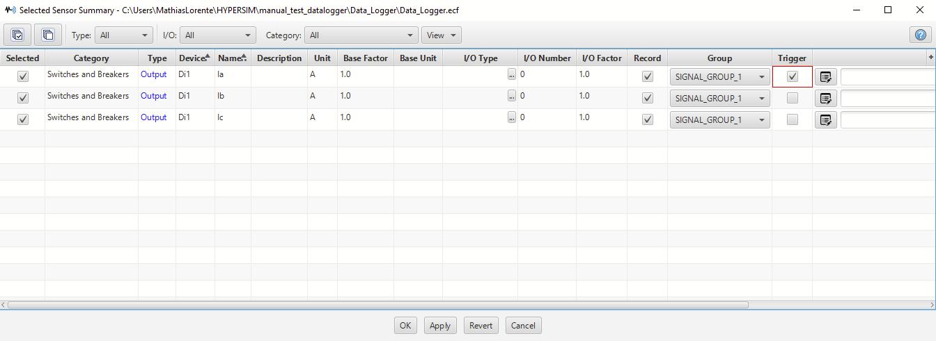
To configure the trigger, check the box in the data logger window. In this scenarios, the triggered signal is the current Ia through Di1.
You can set up different parameters such as:
- Trigger level: Level value that will activate the trigger.
- Trigger function: The trigger is active on an edge or level event.
- Trigger polarity: Negative or positive. When triggering on an edge event, it specifies whether the trigger is to occur on a rising (positive) or falling (negative) edge around the specified trigger value.
- Pre-trigger percentage: Percentage of the record length to be logged before the occurrence of the trigger condition. Example: For 25%, write 25.0.
- Trigger holdoff: After the occurrence of a trigger condition, specifies the duration for which all subsequent trigger events will be ignored. It allows you to record a frame every time that the simulation matches the conditions set in trigger configuration. Uses the unit specified in Frame length units.
Note: Only one trigger per signal group can be set up.
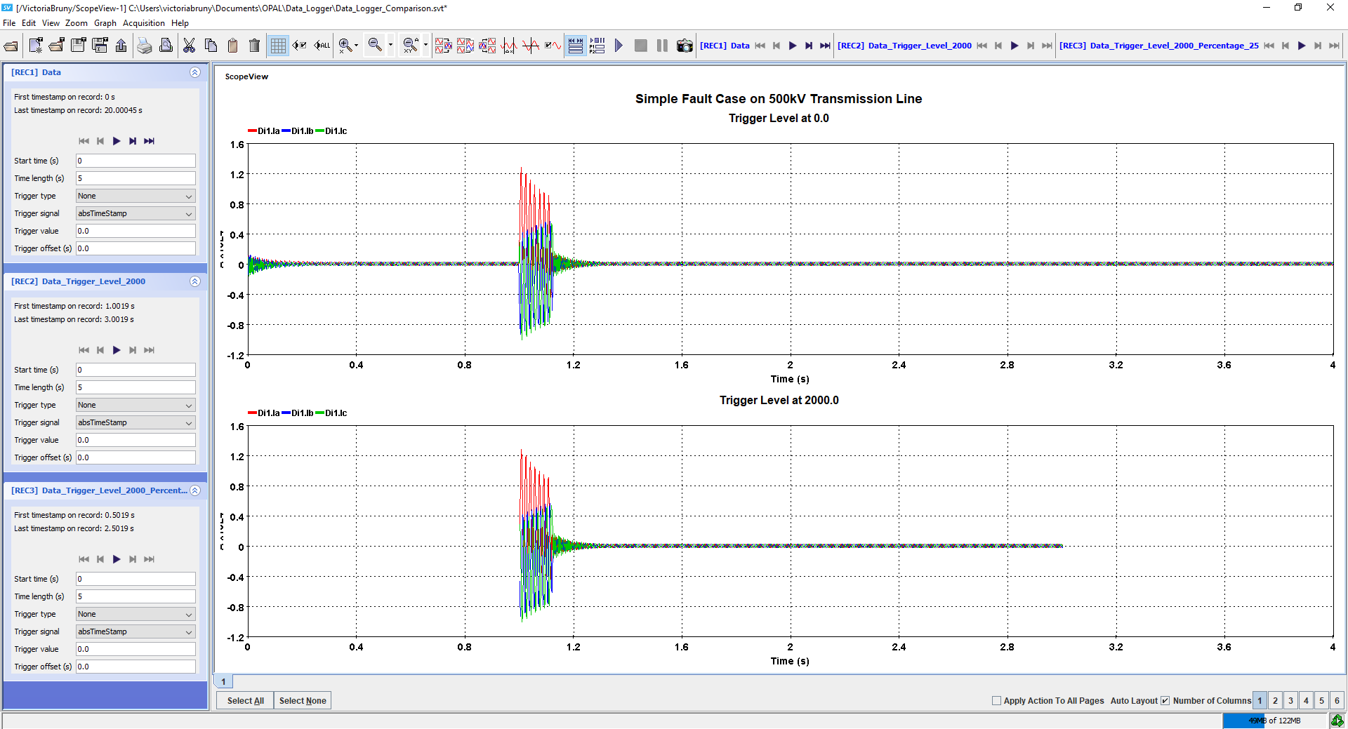
Playing with Trigger Level
Let's compare the acquisition when Trigger Level is at 0.0 and 2000.0.
We can see that below that the acquisition started when Ia crossed 2000.0V.
Note: in this case the data logger recorded only one frame.
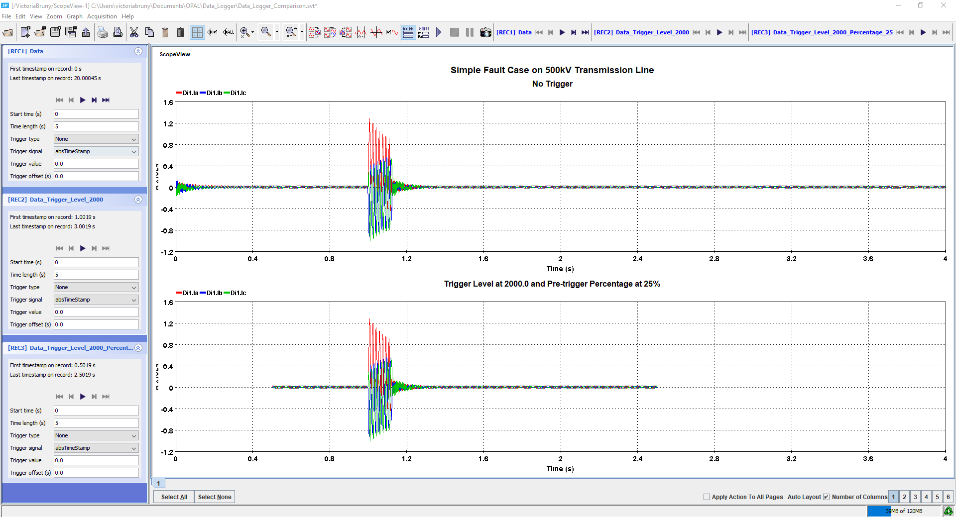
Results
Now we set the Pre-trigger percentage at 25%.
For a frame of 2 seconds, the acquisition started 0.5s before Ia reached 2000.0 that corresponds to 25% of 2 seconds acquisition.
Results
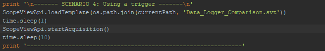
Python Script
Note: This script runs 2 scenarios among 4, 'Recording in Automatic Mode' on the fly and 'Using a trigger' with pre-recorded .oprec files.
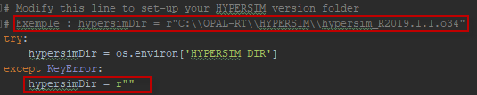
- Before running the script you need to edit "hypersimDir"
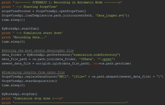
- At this step we run the simulation and record in automatic mode
it opens ScopeView template and display the results of the .oprec file in ScopeView. the waveforms should be the same depending on how long run the simulation in the script.
Results

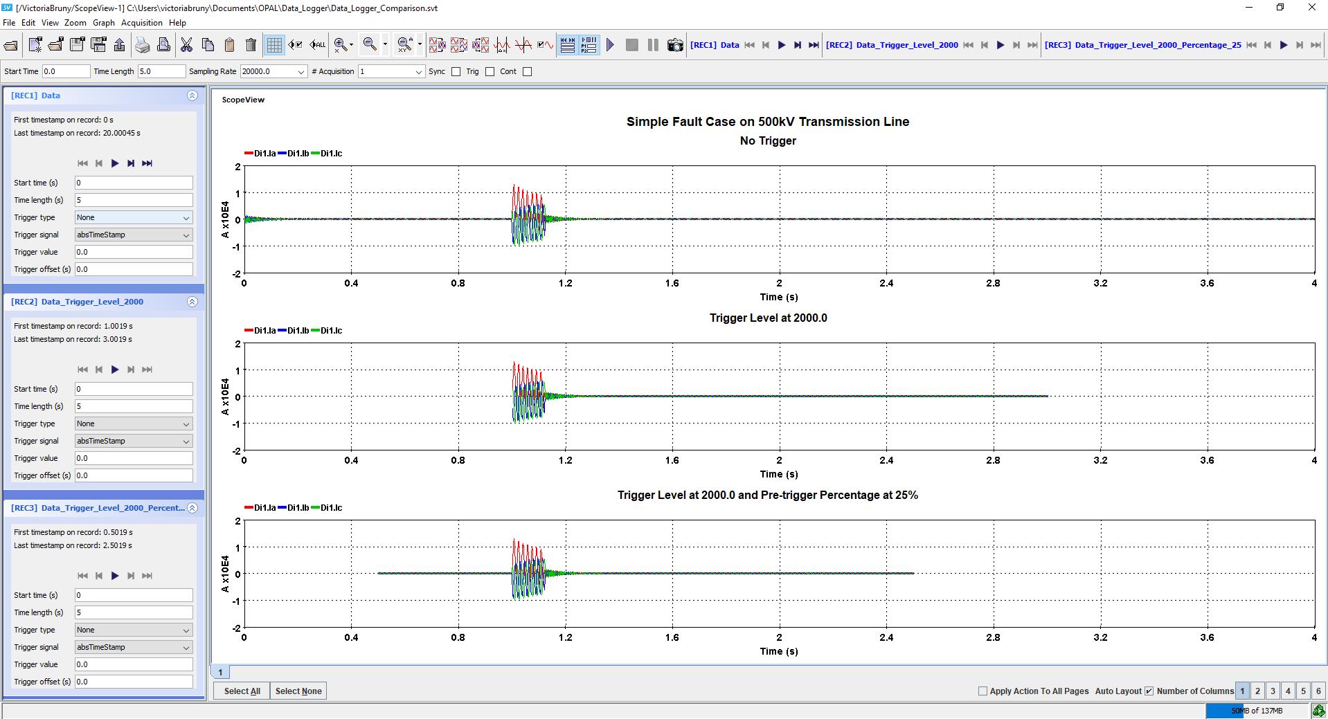
- At this step we compare the waveform depending on the trigger setting of the data logger
ScopeView template has changed and shows 3 different graphs, one without trigger, one with a trigger level at 2000.0V on Di1.Ia and the third one with a trigger level at 2000.0V and a pre-trigger percentage of 25%.
Results
OPAL-RT TECHNOLOGIES, Inc. | 1751, rue Richardson, bureau 1060 | Montréal, Québec Canada H3K 1G6 | opal-rt.com | +1 514-935-2323