Documentation Home Page ◇ HYPERSIM Home Page
Pour la documentation en FRANÇAIS, utilisez l'outil de traduction de votre navigateur Chrome, Edge ou Safari. Voir un exemple.
Examples | Directional Overcurrent Protection
- Sylvain Ménard
Location
This example model can be found in the software under the Protection > Directional_Overcurrent.ecf.
Model Description
Protection systems help in the safe operation of a power network by isolating the faulted section through breakers. The relays within that section respond in a coordinated fashion to achieve high selectivity. While the majority of the relays in the existing network are non-directional, there are certain cases where direction-based discrimination is required to determine if a relay should respond or not. The co-ordinated response of relays along with directionality ensures the safe operation of the network and minimizes service interruptions. Directional overcurrent protection relays are very useful in this regard.
Directional overcurrent protection is used to protect the system when fault currents could circulate in either direction along the network line. With the increasing penetration of Distributed Generation (DG) sources at the distribution network, it becomes even more important to implement directional protection to provide correct fault detection and ensure protection co-ordination.
This example demonstrates the operation of the Directional Overcurrent (505167) relay.
Some assumptions:
In this example, the fuses, reclosers, and sectionalisers are not implemented. The lateral lines are protected by the main-line directional overcurrent relays.
DG protection is also not discussed in this example. The focus is on feeder protection.
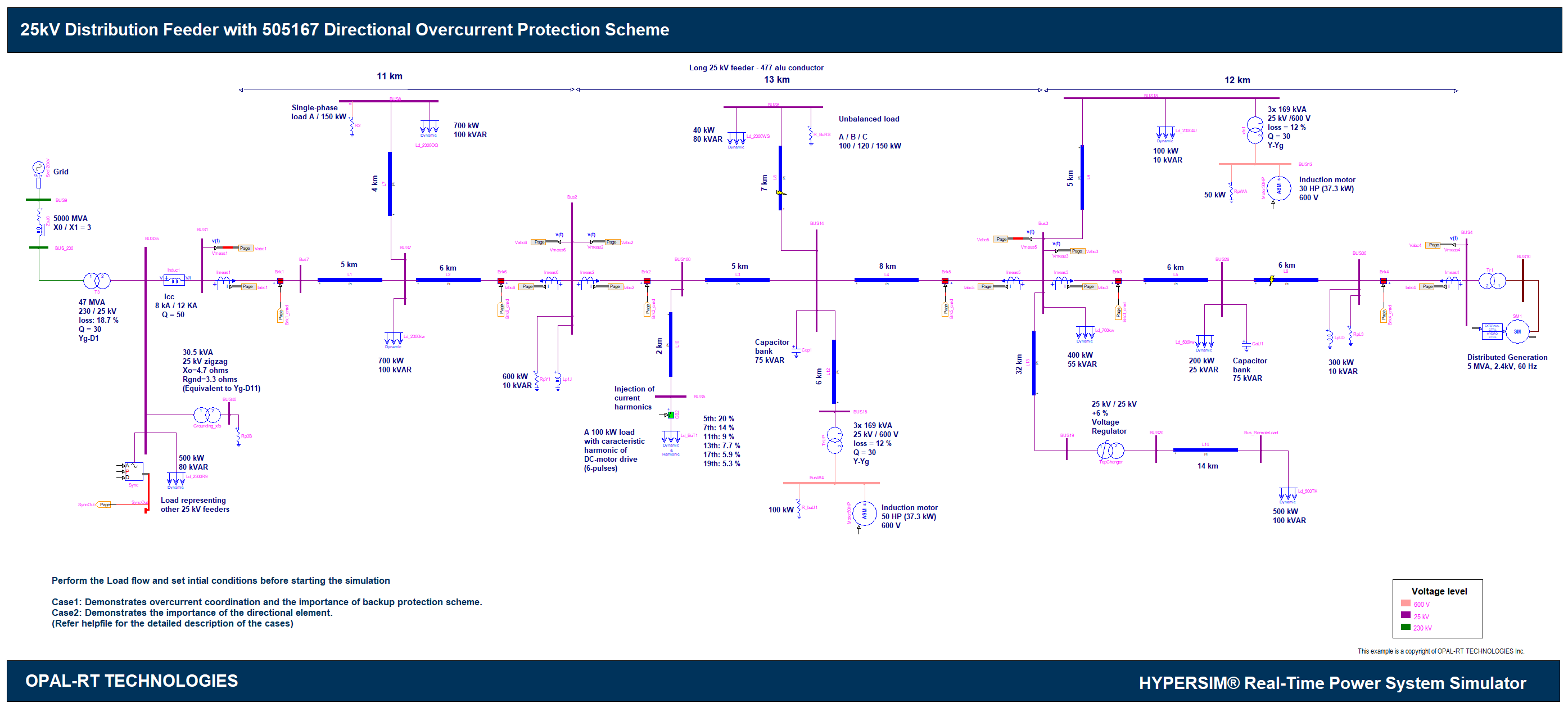
Network Description
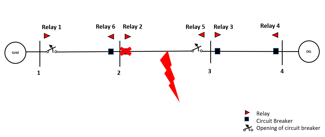
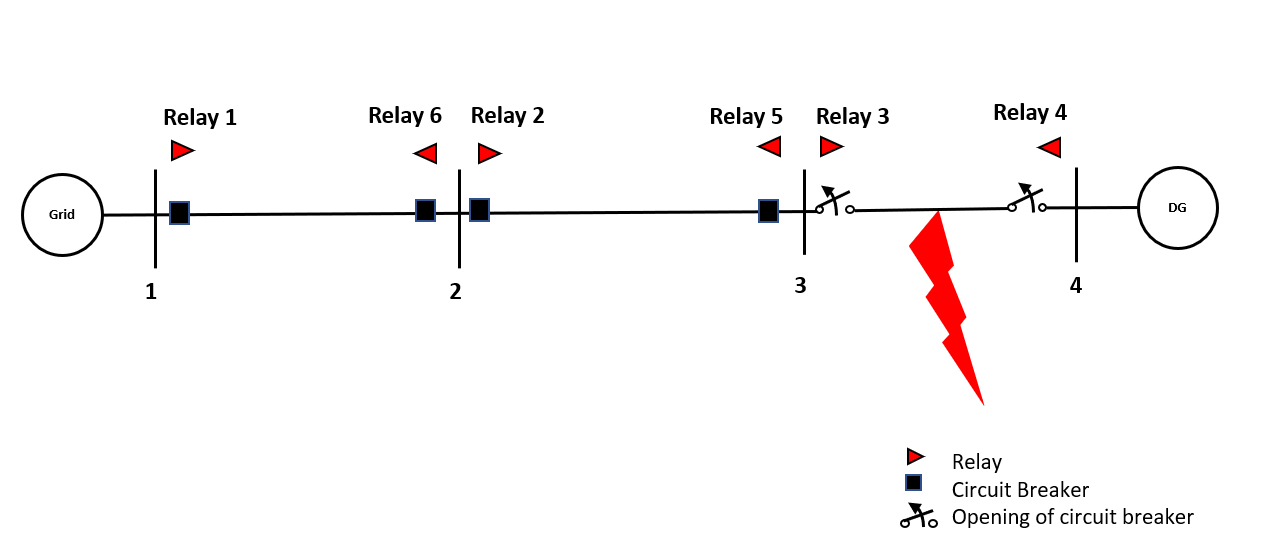
A 25 kV, 60Hz distribution feeder is used as an example for demonstrating the directional overcurrent protection relay operation. The network has two generating sources: an upstream grid modeled as a voltage source and a 5 MVA, 2.4 kV DG (modeled as a synchronous machine) connected at the other end of the feeder through a 2.4 kV / 25 kV (Delta lead- Star grounded) transformer. The DG is operating at 1.8 MW and is operating in the PV mode. The network comprises of a diversity of loads such as dynamic loads, unbalanced loads, induction motors, etc. The schematic of the system is shown in the figure above.
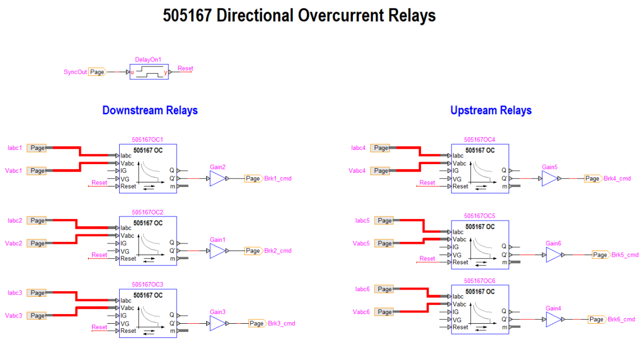
The Current Transformer (CT) and Voltage Transformer (VT) are emulated by the current and voltage measurement sensors respectively. CTs and VTs ratios are selected as 100 A / 1 A and 25 kV / 110 V respectively. The figure below shows the page 2 of the model with the sensor measurements connected to the directional overcurrent protection (505167) relays.
The complete network is divided into three sections 1,2 and 3. The directional overcurrent (505167) relays in the different sections are configured as shown in the figure and table below.
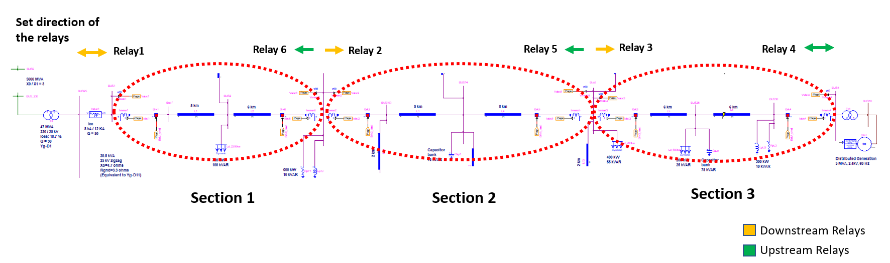
| Relay | Directional/Non-Directional | Set direction | |
|---|---|---|---|
| Downstream Relays | 1 | Non-directional | - |
| 2 | Directional | Left to Right | |
| 3 | Directional | Left to Right | |
| Upstream Relays | 4 | Non-directional | - |
| 5 | Directional | Right to Left | |
| 6 | Directional | Right to Left |
Relay Parameters
Directional Settings
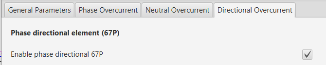
In relays 2, 3, 5 and 6 the directional element (67P) is enabled by checking the 'Enable phase directional 67P'. Element Characteristic Angle (ECA) is selected as 30 deg as shown below:
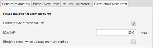
Whereas in relays 1 and 4, the directional element (67P) is disabled.
Coordination of the Relays
Coordination of the Downstream Relays
The table below shows the parameters of the downstream relays, and the methodology of time dial calculation is followed:
| Relay | Base Current (A) | Base Voltage (V) | 51P Pickup current (pu) | Time Dial (s) | Curve Type |
|---|---|---|---|---|---|
| 1 | 0.59 | 65.508 | 2.0 | 0.418 | U.S. Inverse (U2) |
| 2 | 0.18 | 65.508 | 2.2 | 0.286 | U.S. Inverse (U2) |
| 3 | 0.29 | 65.508 | 1.3 | 0.04 | U.S. Inverse (U2) |
In general, the pickup current for the relay is selected such that: 1.2 Ifull_load < Ipickup < 1/3 Imin_Fault
Operating time using U.S. Inverse (U2) as per IEEE C37.112-2018 is given as:
%5e%7b2%7d-1%7d%5cright )%5cend%7barray%7d%3c/title%3e %3cdefs aria-hidden='true'%3e %3cpath stroke-width='1' id='E1-MJMATHI-74' d='M26 385Q19 392 19 395Q19 399 22 411T27 425Q29 430 36 430T87 431H140L159 511Q162 522 166 540T173 566T179 586T187 603T197 615T211 624T229 626Q247 625 254 615T261 596Q261 589 252 549T232 470L222 433Q222 431 272 431H323Q330 424 330 420Q330 398 317 385H210L174 240Q135 80 135 68Q135 26 162 26Q197 26 230 60T283 144Q285 150 288 151T303 153H307Q322 153 322 145Q322 142 319 133Q314 117 301 95T267 48T216 6T155 -11Q125 -11 98 4T59 56Q57 64 57 83V101L92 241Q127 382 128 383Q128 385 77 385H26Z'%3e%3c/path%3e %3cpath stroke-width='1' id='E1-MJMATHI-4F' d='M740 435Q740 320 676 213T511 42T304 -22Q207 -22 138 35T51 201Q50 209 50 244Q50 346 98 438T227 601Q351 704 476 704Q514 704 524 703Q621 689 680 617T740 435ZM637 476Q637 565 591 615T476 665Q396 665 322 605Q242 542 200 428T157 216Q157 126 200 73T314 19Q404 19 485 98T608 313Q637 408 637 476Z'%3e%3c/path%3e %3cpath stroke-width='1' id='E1-MJMATHI-70' d='M23 287Q24 290 25 295T30 317T40 348T55 381T75 411T101 433T134 442Q209 442 230 378L240 387Q302 442 358 442Q423 442 460 395T497 281Q497 173 421 82T249 -10Q227 -10 210 -4Q199 1 187 11T168 28L161 36Q160 35 139 -51T118 -138Q118 -144 126 -145T163 -148H188Q194 -155 194 -157T191 -175Q188 -187 185 -190T172 -194Q170 -194 161 -194T127 -193T65 -192Q-5 -192 -24 -194H-32Q-39 -187 -39 -183Q-37 -156 -26 -148H-6Q28 -147 33 -136Q36 -130 94 103T155 350Q156 355 156 364Q156 405 131 405Q109 405 94 377T71 316T59 280Q57 278 43 278H29Q23 284 23 287ZM178 102Q200 26 252 26Q282 26 310 49T356 107Q374 141 392 215T411 325V331Q411 405 350 405Q339 405 328 402T306 393T286 380T269 365T254 350T243 336T235 326L232 322Q232 321 229 308T218 264T204 212Q178 106 178 102Z'%3e%3c/path%3e %3cpath stroke-width='1' id='E1-MJMATHI-65' d='M39 168Q39 225 58 272T107 350T174 402T244 433T307 442H310Q355 442 388 420T421 355Q421 265 310 237Q261 224 176 223Q139 223 138 221Q138 219 132 186T125 128Q125 81 146 54T209 26T302 45T394 111Q403 121 406 121Q410 121 419 112T429 98T420 82T390 55T344 24T281 -1T205 -11Q126 -11 83 42T39 168ZM373 353Q367 405 305 405Q272 405 244 391T199 357T170 316T154 280T149 261Q149 260 169 260Q282 260 327 284T373 353Z'%3e%3c/path%3e %3cpath stroke-width='1' id='E1-MJMATHI-72' d='M21 287Q22 290 23 295T28 317T38 348T53 381T73 411T99 433T132 442Q161 442 183 430T214 408T225 388Q227 382 228 382T236 389Q284 441 347 441H350Q398 441 422 400Q430 381 430 363Q430 333 417 315T391 292T366 288Q346 288 334 299T322 328Q322 376 378 392Q356 405 342 405Q286 405 239 331Q229 315 224 298T190 165Q156 25 151 16Q138 -11 108 -11Q95 -11 87 -5T76 7T74 17Q74 30 114 189T154 366Q154 405 128 405Q107 405 92 377T68 316T57 280Q55 278 41 278H27Q21 284 21 287Z'%3e%3c/path%3e %3cpath stroke-width='1' id='E1-MJMATHI-61' d='M33 157Q33 258 109 349T280 441Q331 441 370 392Q386 422 416 422Q429 422 439 414T449 394Q449 381 412 234T374 68Q374 43 381 35T402 26Q411 27 422 35Q443 55 463 131Q469 151 473 152Q475 153 483 153H487Q506 153 506 144Q506 138 501 117T481 63T449 13Q436 0 417 -8Q409 -10 393 -10Q359 -10 336 5T306 36L300 51Q299 52 296 50Q294 48 292 46Q233 -10 172 -10Q117 -10 75 30T33 157ZM351 328Q351 334 346 350T323 385T277 405Q242 405 210 374T160 293Q131 214 119 129Q119 126 119 118T118 106Q118 61 136 44T179 26Q217 26 254 59T298 110Q300 114 325 217T351 328Z'%3e%3c/path%3e %3cpath stroke-width='1' id='E1-MJMATHI-69' d='M184 600Q184 624 203 642T247 661Q265 661 277 649T290 619Q290 596 270 577T226 557Q211 557 198 567T184 600ZM21 287Q21 295 30 318T54 369T98 420T158 442Q197 442 223 419T250 357Q250 340 236 301T196 196T154 83Q149 61 149 51Q149 26 166 26Q175 26 185 29T208 43T235 78T260 137Q263 149 265 151T282 153Q302 153 302 143Q302 135 293 112T268 61T223 11T161 -11Q129 -11 102 10T74 74Q74 91 79 106T122 220Q160 321 166 341T173 380Q173 404 156 404H154Q124 404 99 371T61 287Q60 286 59 284T58 281T56 279T53 278T49 278T41 278H27Q21 284 21 287Z'%3e%3c/path%3e %3cpath stroke-width='1' id='E1-MJMATHI-6F' d='M201 -11Q126 -11 80 38T34 156Q34 221 64 279T146 380Q222 441 301 441Q333 441 341 440Q354 437 367 433T402 417T438 387T464 338T476 268Q476 161 390 75T201 -11ZM121 120Q121 70 147 48T206 26Q250 26 289 58T351 142Q360 163 374 216T388 308Q388 352 370 375Q346 405 306 405Q243 405 195 347Q158 303 140 230T121 120Z'%3e%3c/path%3e %3cpath stroke-width='1' id='E1-MJMATHI-6E' d='M21 287Q22 293 24 303T36 341T56 388T89 425T135 442Q171 442 195 424T225 390T231 369Q231 367 232 367L243 378Q304 442 382 442Q436 442 469 415T503 336T465 179T427 52Q427 26 444 26Q450 26 453 27Q482 32 505 65T540 145Q542 153 560 153Q580 153 580 145Q580 144 576 130Q568 101 554 73T508 17T439 -10Q392 -10 371 17T350 73Q350 92 386 193T423 345Q423 404 379 404H374Q288 404 229 303L222 291L189 157Q156 26 151 16Q138 -11 108 -11Q95 -11 87 -5T76 7T74 17Q74 30 112 180T152 343Q153 348 153 366Q153 405 129 405Q91 405 66 305Q60 285 60 284Q58 278 41 278H27Q21 284 21 287Z'%3e%3c/path%3e %3cpath stroke-width='1' id='E1-MJMAIN-3D' d='M56 347Q56 360 70 367H707Q722 359 722 347Q722 336 708 328L390 327H72Q56 332 56 347ZM56 153Q56 168 72 173H708Q722 163 722 153Q722 140 707 133H70Q56 140 56 153Z'%3e%3c/path%3e %3cpath stroke-width='1' id='E1-MJMATHI-54' d='M40 437Q21 437 21 445Q21 450 37 501T71 602L88 651Q93 669 101 677H569H659Q691 677 697 676T704 667Q704 661 687 553T668 444Q668 437 649 437Q640 437 637 437T631 442L629 445Q629 451 635 490T641 551Q641 586 628 604T573 629Q568 630 515 631Q469 631 457 630T439 622Q438 621 368 343T298 60Q298 48 386 46Q418 46 427 45T436 36Q436 31 433 22Q429 4 424 1L422 0Q419 0 415 0Q410 0 363 1T228 2Q99 2 64 0H49Q43 6 43 9T45 27Q49 40 55 46H83H94Q174 46 189 55Q190 56 191 56Q196 59 201 76T241 233Q258 301 269 344Q339 619 339 625Q339 630 310 630H279Q212 630 191 624Q146 614 121 583T67 467Q60 445 57 441T43 437H40Z'%3e%3c/path%3e %3cpath stroke-width='1' id='E1-MJMAIN-2E' d='M78 60Q78 84 95 102T138 120Q162 120 180 104T199 61Q199 36 182 18T139 0T96 17T78 60Z'%3e%3c/path%3e %3cpath stroke-width='1' id='E1-MJMATHI-44' d='M287 628Q287 635 230 637Q207 637 200 638T193 647Q193 655 197 667T204 682Q206 683 403 683Q570 682 590 682T630 676Q702 659 752 597T803 431Q803 275 696 151T444 3L430 1L236 0H125H72Q48 0 41 2T33 11Q33 13 36 25Q40 41 44 43T67 46Q94 46 127 49Q141 52 146 61Q149 65 218 339T287 628ZM703 469Q703 507 692 537T666 584T629 613T590 629T555 636Q553 636 541 636T512 636T479 637H436Q392 637 386 627Q384 623 313 339T242 52Q242 48 253 48T330 47Q335 47 349 47T373 46Q499 46 581 128Q617 164 640 212T683 339T703 469Z'%3e%3c/path%3e %3cpath stroke-width='1' id='E1-MJMAIN-2217' d='M229 286Q216 420 216 436Q216 454 240 464Q241 464 245 464T251 465Q263 464 273 456T283 436Q283 419 277 356T270 286L328 328Q384 369 389 372T399 375Q412 375 423 365T435 338Q435 325 425 315Q420 312 357 282T289 250L355 219L425 184Q434 175 434 161Q434 146 425 136T401 125Q393 125 383 131T328 171L270 213Q283 79 283 63Q283 53 276 44T250 35Q231 35 224 44T216 63Q216 80 222 143T229 213L171 171Q115 130 110 127Q106 124 100 124Q87 124 76 134T64 161Q64 166 64 169T67 175T72 181T81 188T94 195T113 204T138 215T170 230T210 250L74 315Q65 324 65 338Q65 353 74 363T98 374Q106 374 116 368T171 328L229 286Z'%3e%3c/path%3e %3cpath stroke-width='1' id='E1-MJMAIN-28' d='M94 250Q94 319 104 381T127 488T164 576T202 643T244 695T277 729T302 750H315H319Q333 750 333 741Q333 738 316 720T275 667T226 581T184 443T167 250T184 58T225 -81T274 -167T316 -220T333 -241Q333 -250 318 -250H315H302L274 -226Q180 -141 137 -14T94 250Z'%3e%3c/path%3e %3cpath stroke-width='1' id='E1-MJMAIN-30' d='M96 585Q152 666 249 666Q297 666 345 640T423 548Q460 465 460 320Q460 165 417 83Q397 41 362 16T301 -15T250 -22Q224 -22 198 -16T137 16T82 83Q39 165 39 320Q39 494 96 585ZM321 597Q291 629 250 629Q208 629 178 597Q153 571 145 525T137 333Q137 175 145 125T181 46Q209 16 250 16Q290 16 318 46Q347 76 354 130T362 333Q362 478 354 524T321 597Z'%3e%3c/path%3e %3cpath stroke-width='1' id='E1-MJMAIN-31' d='M213 578L200 573Q186 568 160 563T102 556H83V602H102Q149 604 189 617T245 641T273 663Q275 666 285 666Q294 666 302 660V361L303 61Q310 54 315 52T339 48T401 46H427V0H416Q395 3 257 3Q121 3 100 0H88V46H114Q136 46 152 46T177 47T193 50T201 52T207 57T213 61V578Z'%3e%3c/path%3e %3cpath stroke-width='1' id='E1-MJMAIN-38' d='M70 417T70 494T124 618T248 666Q319 666 374 624T429 515Q429 485 418 459T392 417T361 389T335 371T324 363L338 354Q352 344 366 334T382 323Q457 264 457 174Q457 95 399 37T249 -22Q159 -22 101 29T43 155Q43 263 172 335L154 348Q133 361 127 368Q70 417 70 494ZM286 386L292 390Q298 394 301 396T311 403T323 413T334 425T345 438T355 454T364 471T369 491T371 513Q371 556 342 586T275 624Q268 625 242 625Q201 625 165 599T128 534Q128 511 141 492T167 463T217 431Q224 426 228 424L286 386ZM250 21Q308 21 350 55T392 137Q392 154 387 169T375 194T353 216T330 234T301 253T274 270Q260 279 244 289T218 306L210 311Q204 311 181 294T133 239T107 157Q107 98 150 60T250 21Z'%3e%3c/path%3e %3cpath stroke-width='1' id='E1-MJMAIN-2B' d='M56 237T56 250T70 270H369V420L370 570Q380 583 389 583Q402 583 409 568V270H707Q722 262 722 250T707 230H409V-68Q401 -82 391 -82H389H387Q375 -82 369 -68V230H70Q56 237 56 250Z'%3e%3c/path%3e %3cpath stroke-width='1' id='E1-MJMAIN-35' d='M164 157Q164 133 148 117T109 101H102Q148 22 224 22Q294 22 326 82Q345 115 345 210Q345 313 318 349Q292 382 260 382H254Q176 382 136 314Q132 307 129 306T114 304Q97 304 95 310Q93 314 93 485V614Q93 664 98 664Q100 666 102 666Q103 666 123 658T178 642T253 634Q324 634 389 662Q397 666 402 666Q410 666 410 648V635Q328 538 205 538Q174 538 149 544L139 546V374Q158 388 169 396T205 412T256 420Q337 420 393 355T449 201Q449 109 385 44T229 -22Q148 -22 99 32T50 154Q50 178 61 192T84 210T107 214Q132 214 148 197T164 157Z'%3e%3c/path%3e %3cpath stroke-width='1' id='E1-MJMAIN-39' d='M352 287Q304 211 232 211Q154 211 104 270T44 396Q42 412 42 436V444Q42 537 111 606Q171 666 243 666Q245 666 249 666T257 665H261Q273 665 286 663T323 651T370 619T413 560Q456 472 456 334Q456 194 396 97Q361 41 312 10T208 -22Q147 -22 108 7T68 93T121 149Q143 149 158 135T173 96Q173 78 164 65T148 49T135 44L131 43Q131 41 138 37T164 27T206 22H212Q272 22 313 86Q352 142 352 280V287ZM244 248Q292 248 321 297T351 430Q351 508 343 542Q341 552 337 562T323 588T293 615T246 625Q208 625 181 598Q160 576 154 546T147 441Q147 358 152 329T172 282Q197 248 244 248Z'%3e%3c/path%3e %3cpath stroke-width='1' id='E1-MJMATHI-49' d='M43 1Q26 1 26 10Q26 12 29 24Q34 43 39 45Q42 46 54 46H60Q120 46 136 53Q137 53 138 54Q143 56 149 77T198 273Q210 318 216 344Q286 624 286 626Q284 630 284 631Q274 637 213 637H193Q184 643 189 662Q193 677 195 680T209 683H213Q285 681 359 681Q481 681 487 683H497Q504 676 504 672T501 655T494 639Q491 637 471 637Q440 637 407 634Q393 631 388 623Q381 609 337 432Q326 385 315 341Q245 65 245 59Q245 52 255 50T307 46H339Q345 38 345 37T342 19Q338 6 332 0H316Q279 2 179 2Q143 2 113 2T65 2T43 1Z'%3e%3c/path%3e %3cpath stroke-width='1' id='E1-MJMATHI-66' d='M118 -162Q120 -162 124 -164T135 -167T147 -168Q160 -168 171 -155T187 -126Q197 -99 221 27T267 267T289 382V385H242Q195 385 192 387Q188 390 188 397L195 425Q197 430 203 430T250 431Q298 431 298 432Q298 434 307 482T319 540Q356 705 465 705Q502 703 526 683T550 630Q550 594 529 578T487 561Q443 561 443 603Q443 622 454 636T478 657L487 662Q471 668 457 668Q445 668 434 658T419 630Q412 601 403 552T387 469T380 433Q380 431 435 431Q480 431 487 430T498 424Q499 420 496 407T491 391Q489 386 482 386T428 385H372L349 263Q301 15 282 -47Q255 -132 212 -173Q175 -205 139 -205Q107 -205 81 -186T55 -132Q55 -95 76 -78T118 -61Q162 -61 162 -103Q162 -122 151 -136T127 -157L118 -162Z'%3e%3c/path%3e %3cpath stroke-width='1' id='E1-MJMATHI-75' d='M21 287Q21 295 30 318T55 370T99 420T158 442Q204 442 227 417T250 358Q250 340 216 246T182 105Q182 62 196 45T238 27T291 44T328 78L339 95Q341 99 377 247Q407 367 413 387T427 416Q444 431 463 431Q480 431 488 421T496 402L420 84Q419 79 419 68Q419 43 426 35T447 26Q469 29 482 57T512 145Q514 153 532 153Q551 153 551 144Q550 139 549 130T540 98T523 55T498 17T462 -8Q454 -10 438 -10Q372 -10 347 46Q345 45 336 36T318 21T296 6T267 -6T233 -11Q189 -11 155 7Q103 38 103 113Q103 170 138 262T173 379Q173 380 173 381Q173 390 173 393T169 400T158 404H154Q131 404 112 385T82 344T65 302T57 280Q55 278 41 278H27Q21 284 21 287Z'%3e%3c/path%3e %3cpath stroke-width='1' id='E1-MJMATHI-6C' d='M117 59Q117 26 142 26Q179 26 205 131Q211 151 215 152Q217 153 225 153H229Q238 153 241 153T246 151T248 144Q247 138 245 128T234 90T214 43T183 6T137 -11Q101 -11 70 11T38 85Q38 97 39 102L104 360Q167 615 167 623Q167 626 166 628T162 632T157 634T149 635T141 636T132 637T122 637Q112 637 109 637T101 638T95 641T94 647Q94 649 96 661Q101 680 107 682T179 688Q194 689 213 690T243 693T254 694Q266 694 266 686Q266 675 193 386T118 83Q118 81 118 75T117 65V59Z'%3e%3c/path%3e %3cpath stroke-width='1' id='E1-MJMATHI-63' d='M34 159Q34 268 120 355T306 442Q362 442 394 418T427 355Q427 326 408 306T360 285Q341 285 330 295T319 325T330 359T352 380T366 386H367Q367 388 361 392T340 400T306 404Q276 404 249 390Q228 381 206 359Q162 315 142 235T121 119Q121 73 147 50Q169 26 205 26H209Q321 26 394 111Q403 121 406 121Q410 121 419 112T429 98T420 83T391 55T346 25T282 0T202 -11Q127 -11 81 37T34 159Z'%3e%3c/path%3e %3cpath stroke-width='1' id='E1-MJMATHI-6B' d='M121 647Q121 657 125 670T137 683Q138 683 209 688T282 694Q294 694 294 686Q294 679 244 477Q194 279 194 272Q213 282 223 291Q247 309 292 354T362 415Q402 442 438 442Q468 442 485 423T503 369Q503 344 496 327T477 302T456 291T438 288Q418 288 406 299T394 328Q394 353 410 369T442 390L458 393Q446 405 434 405H430Q398 402 367 380T294 316T228 255Q230 254 243 252T267 246T293 238T320 224T342 206T359 180T365 147Q365 130 360 106T354 66Q354 26 381 26Q429 26 459 145Q461 153 479 153H483Q499 153 499 144Q499 139 496 130Q455 -11 378 -11Q333 -11 305 15T277 90Q277 108 280 121T283 145Q283 167 269 183T234 206T200 217T182 220H180Q168 178 159 139T145 81T136 44T129 20T122 7T111 -2Q98 -11 83 -11Q66 -11 57 -1T48 16Q48 26 85 176T158 471L195 616Q196 629 188 632T149 637H144Q134 637 131 637T124 640T121 647Z'%3e%3c/path%3e %3cpath stroke-width='1' id='E1-MJMAIN-29' d='M60 749L64 750Q69 750 74 750H86L114 726Q208 641 251 514T294 250Q294 182 284 119T261 12T224 -76T186 -143T145 -194T113 -227T90 -246Q87 -249 86 -250H74Q66 -250 63 -250T58 -247T55 -238Q56 -237 66 -225Q221 -64 221 250T66 725Q56 737 55 738Q55 746 60 749Z'%3e%3c/path%3e %3cpath stroke-width='1' id='E1-MJSZ2-28' d='M180 96T180 250T205 541T266 770T353 944T444 1069T527 1150H555Q561 1144 561 1141Q561 1137 545 1120T504 1072T447 995T386 878T330 721T288 513T272 251Q272 133 280 56Q293 -87 326 -209T399 -405T475 -531T536 -609T561 -640Q561 -643 555 -649H527Q483 -612 443 -568T353 -443T266 -270T205 -41Z'%3e%3c/path%3e %3cpath stroke-width='1' id='E1-MJSZ2-29' d='M35 1138Q35 1150 51 1150H56H69Q113 1113 153 1069T243 944T330 771T391 541T416 250T391 -40T330 -270T243 -443T152 -568T69 -649H56Q43 -649 39 -647T35 -637Q65 -607 110 -548Q283 -316 316 56Q324 133 324 251Q324 368 316 445Q278 877 48 1123Q36 1137 35 1138Z'%3e%3c/path%3e %3cpath stroke-width='1' id='E1-MJMAIN-32' d='M109 429Q82 429 66 447T50 491Q50 562 103 614T235 666Q326 666 387 610T449 465Q449 422 429 383T381 315T301 241Q265 210 201 149L142 93L218 92Q375 92 385 97Q392 99 409 186V189H449V186Q448 183 436 95T421 3V0H50V19V31Q50 38 56 46T86 81Q115 113 136 137Q145 147 170 174T204 211T233 244T261 278T284 308T305 340T320 369T333 401T340 431T343 464Q343 527 309 573T212 619Q179 619 154 602T119 569T109 550Q109 549 114 549Q132 549 151 535T170 489Q170 464 154 447T109 429Z'%3e%3c/path%3e %3cpath stroke-width='1' id='E1-MJMAIN-2212' d='M84 237T84 250T98 270H679Q694 262 694 250T679 230H98Q84 237 84 250Z'%3e%3c/path%3e %3cpath stroke-width='1' id='E1-MJSZ4-239B' d='M837 1154Q843 1148 843 1145Q843 1141 818 1106T753 1002T667 841T574 604T494 299Q417 -84 417 -609Q417 -641 416 -647T411 -654Q409 -655 366 -655Q299 -655 297 -654Q292 -652 292 -643T291 -583Q293 -400 304 -242T347 110T432 470T574 813T785 1136Q787 1139 790 1142T794 1147T796 1150T799 1152T802 1153T807 1154T813 1154H819H837Z'%3e%3c/path%3e %3cpath stroke-width='1' id='E1-MJSZ4-239D' d='M843 -635Q843 -638 837 -644H820Q801 -644 800 -643Q792 -635 785 -626Q684 -503 605 -363T473 -75T385 216T330 518T302 809T291 1093Q291 1144 291 1153T296 1164Q298 1165 366 1165Q409 1165 411 1164Q415 1163 416 1157T417 1119Q417 529 517 109T833 -617Q843 -631 843 -635Z'%3e%3c/path%3e %3cpath stroke-width='1' id='E1-MJSZ4-239C' d='M413 -9Q412 -9 407 -9T388 -10T354 -10Q300 -10 297 -9Q294 -8 293 -5Q291 5 291 127V300Q291 602 292 605L296 609Q298 610 366 610Q382 610 392 610T407 610T412 609Q416 609 416 592T417 473V127Q417 -9 413 -9Z'%3e%3c/path%3e %3cpath stroke-width='1' id='E1-MJSZ4-239E' d='M31 1143Q31 1154 49 1154H59Q72 1154 75 1152T89 1136Q190 1013 269 873T401 585T489 294T544 -8T572 -299T583 -583Q583 -634 583 -643T577 -654Q575 -655 508 -655Q465 -655 463 -654Q459 -653 458 -647T457 -609Q457 -58 371 340T100 1037Q87 1059 61 1098T31 1143Z'%3e%3c/path%3e %3cpath stroke-width='1' id='E1-MJSZ4-23A0' d='M56 -644H50Q31 -644 31 -635Q31 -632 37 -622Q69 -579 100 -527Q286 -228 371 170T457 1119Q457 1161 462 1164Q464 1165 520 1165Q575 1165 577 1164Q582 1162 582 1153T583 1093Q581 910 570 752T527 400T442 40T300 -303T89 -626Q78 -640 75 -642T61 -644H56Z'%3e%3c/path%3e %3cpath stroke-width='1' id='E1-MJSZ4-239F' d='M579 -9Q578 -9 573 -9T554 -10T520 -10Q466 -10 463 -9Q460 -8 459 -5Q457 5 457 127V300Q457 602 458 605L462 609Q464 610 532 610Q548 610 558 610T573 610T578 609Q582 609 582 592T583 473V127Q583 -9 579 -9Z'%3e%3c/path%3e %3c/defs%3e %3cg stroke='currentColor' fill='currentColor' stroke-width='0' transform='matrix(1 0 0 -1 0 0)' aria-hidden='true'%3e %3cg transform='translate(167%2c0)'%3e %3cg transform='translate(-11%2c0)'%3e %3cuse xlink:href='%23E1-MJMATHI-74' x='0' y='0'%3e%3c/use%3e %3cg transform='translate(361%2c-155)'%3e %3cuse transform='scale(0.707)' xlink:href='%23E1-MJMATHI-4F' x='0' y='0'%3e%3c/use%3e %3cuse transform='scale(0.707)' xlink:href='%23E1-MJMATHI-70' x='763' y='0'%3e%3c/use%3e %3cuse transform='scale(0.707)' xlink:href='%23E1-MJMATHI-65' x='1267' y='0'%3e%3c/use%3e %3cuse transform='scale(0.707)' xlink:href='%23E1-MJMATHI-72' x='1733' y='0'%3e%3c/use%3e %3cuse transform='scale(0.707)' xlink:href='%23E1-MJMATHI-61' x='2185' y='0'%3e%3c/use%3e %3cuse transform='scale(0.707)' xlink:href='%23E1-MJMATHI-74' x='2714' y='0'%3e%3c/use%3e %3cuse transform='scale(0.707)' xlink:href='%23E1-MJMATHI-69' x='3076' y='0'%3e%3c/use%3e %3cuse transform='scale(0.707)' xlink:href='%23E1-MJMATHI-6F' x='3421' y='0'%3e%3c/use%3e %3cuse transform='scale(0.707)' xlink:href='%23E1-MJMATHI-6E' x='3907' y='0'%3e%3c/use%3e %3c/g%3e %3cuse xlink:href='%23E1-MJMAIN-3D' x='3926' y='0'%3e%3c/use%3e %3cuse xlink:href='%23E1-MJMATHI-54' x='4982' y='0'%3e%3c/use%3e %3cuse xlink:href='%23E1-MJMAIN-2E' x='5687' y='0'%3e%3c/use%3e %3cuse xlink:href='%23E1-MJMATHI-44' x='6132' y='0'%3e%3c/use%3e %3cuse xlink:href='%23E1-MJMAIN-2E' x='6961' y='0'%3e%3c/use%3e %3cuse xlink:href='%23E1-MJMAIN-2217' x='7406' y='0'%3e%3c/use%3e %3cg transform='translate(8073%2c0)'%3e %3cg transform='translate(0%2c2621)'%3e %3cuse xlink:href='%23E1-MJSZ4-239B' x='0' y='-1156'%3e%3c/use%3e %3cg transform='translate(0%2c-2959.085251503511) scale(1%2c1.9592229975507542)'%3e %3cuse xlink:href='%23E1-MJSZ4-239C'%3e%3c/use%3e %3c/g%3e %3cuse xlink:href='%23E1-MJSZ4-239D' x='0' y='-4099'%3e%3c/use%3e %3c/g%3e %3cg transform='translate(875%2c0)'%3e %3cuse xlink:href='%23E1-MJMAIN-30'%3e%3c/use%3e %3cuse xlink:href='%23E1-MJMAIN-2E' x='500' y='0'%3e%3c/use%3e %3cuse xlink:href='%23E1-MJMAIN-31' x='779' y='0'%3e%3c/use%3e %3cuse xlink:href='%23E1-MJMAIN-38' x='1279' y='0'%3e%3c/use%3e %3c/g%3e %3cuse xlink:href='%23E1-MJMAIN-2B' x='2877' y='0'%3e%3c/use%3e %3cg transform='translate(3656%2c0)'%3e %3cg transform='translate(342%2c0)'%3e %3crect stroke='none' width='5887' height='60' x='0' y='220'%3e%3c/rect%3e %3cg transform='translate(2053%2c676)'%3e %3cuse xlink:href='%23E1-MJMAIN-35'%3e%3c/use%3e %3cuse xlink:href='%23E1-MJMAIN-2E' x='500' y='0'%3e%3c/use%3e %3cuse xlink:href='%23E1-MJMAIN-39' x='779' y='0'%3e%3c/use%3e %3cuse xlink:href='%23E1-MJMAIN-35' x='1279' y='0'%3e%3c/use%3e %3c/g%3e %3cg transform='translate(60%2c-1427)'%3e %3cuse xlink:href='%23E1-MJSZ2-28'%3e%3c/use%3e %3cg transform='translate(597%2c0)'%3e %3cg transform='translate(120%2c0)'%3e %3crect stroke='none' width='2155' height='60' x='0' y='220'%3e%3c/rect%3e %3cg transform='translate(222%2c724)'%3e %3cuse transform='scale(0.707)' xlink:href='%23E1-MJMATHI-49' x='0' y='0'%3e%3c/use%3e %3cg transform='translate(311%2c-162)'%3e %3cuse transform='scale(0.574)' xlink:href='%23E1-MJMATHI-66' x='0' y='0'%3e%3c/use%3e %3cuse transform='scale(0.574)' xlink:href='%23E1-MJMATHI-61' x='550' y='0'%3e%3c/use%3e %3cuse transform='scale(0.574)' xlink:href='%23E1-MJMATHI-75' x='1080' y='0'%3e%3c/use%3e %3cuse transform='scale(0.574)' xlink:href='%23E1-MJMATHI-6C' x='1652' y='0'%3e%3c/use%3e %3cuse transform='scale(0.574)' xlink:href='%23E1-MJMATHI-74' x='1951' y='0'%3e%3c/use%3e %3c/g%3e %3c/g%3e %3cg transform='translate(60%2c-429)'%3e %3cuse transform='scale(0.707)' xlink:href='%23E1-MJMATHI-49' x='0' y='0'%3e%3c/use%3e %3cg transform='translate(311%2c-156)'%3e %3cuse transform='scale(0.574)' xlink:href='%23E1-MJMATHI-70' x='0' y='0'%3e%3c/use%3e %3cuse transform='scale(0.574)' xlink:href='%23E1-MJMATHI-69' x='503' y='0'%3e%3c/use%3e %3cuse transform='scale(0.574)' xlink:href='%23E1-MJMATHI-63' x='849' y='0'%3e%3c/use%3e %3cuse transform='scale(0.574)' xlink:href='%23E1-MJMATHI-6B' x='1282' y='0'%3e%3c/use%3e %3cuse transform='scale(0.574)' xlink:href='%23E1-MJMATHI-75' x='1804' y='0'%3e%3c/use%3e %3cuse transform='scale(0.574)' xlink:href='%23E1-MJMATHI-70' x='2376' y='0'%3e%3c/use%3e %3c/g%3e %3c/g%3e %3c/g%3e %3c/g%3e %3cuse xlink:href='%23E1-MJSZ2-29' x='2993' y='-1'%3e%3c/use%3e %3cuse transform='scale(0.707)' xlink:href='%23E1-MJMAIN-32' x='5077' y='1322'%3e%3c/use%3e %3cuse xlink:href='%23E1-MJMAIN-2212' x='4266' y='0'%3e%3c/use%3e %3cuse xlink:href='%23E1-MJMAIN-31' x='5267' y='0'%3e%3c/use%3e %3c/g%3e %3c/g%3e %3c/g%3e %3cg transform='translate(10006%2c2621)'%3e %3cuse xlink:href='%23E1-MJSZ4-239E' x='0' y='-1155'%3e%3c/use%3e %3cg transform='translate(0%2c-2959.0659898662716) scale(1%2c1.9608281339873515)'%3e %3cuse xlink:href='%23E1-MJSZ4-239F'%3e%3c/use%3e %3c/g%3e %3cuse xlink:href='%23E1-MJSZ4-23A0' x='0' y='-4099'%3e%3c/use%3e %3c/g%3e %3c/g%3e %3c/g%3e %3c/g%3e %3c/g%3e %3c/svg%3e)
|
where T.D. is the Time Dial setting
Calculation of Time Dial setting
Step 1: In this step, the Time Dial for relay 3 is set.
Choose the lowest value of Time Dial setting for relay 3 (0.04 s). No intentional time delay is provided because it does not have backup responsibility.
For close-in fault (three-phase-to-ground fault close to relay) at relay 3 ( ' aria-hidden='true'%3e %3cg transform='translate(167%2c0)'%3e %3cg transform='translate(-11%2c0)'%3e %3cuse xlink:href='%23E1-MJMATHI-49' x='0' y='0'%3e%3c/use%3e %3cg transform='translate(440%2c-155)'%3e %3cuse transform='scale(0.707)' xlink:href='%23E1-MJMATHI-66' x='0' y='0'%3e%3c/use%3e %3cuse transform='scale(0.707)' xlink:href='%23E1-MJMATHI-61' x='550' y='0'%3e%3c/use%3e %3cuse transform='scale(0.707)' xlink:href='%23E1-MJMATHI-75' x='1080' y='0'%3e%3c/use%3e %3cuse transform='scale(0.707)' xlink:href='%23E1-MJMATHI-6C' x='1652' y='0'%3e%3c/use%3e %3cuse transform='scale(0.707)' xlink:href='%23E1-MJMATHI-74' x='1950' y='0'%3e%3c/use%3e %3c/g%3e %3cuse xlink:href='%23E1-MJMAIN-3D' x='2453' y='0'%3e%3c/use%3e %3cg transform='translate(3509%2c0)'%3e %3cuse xlink:href='%23E1-MJMAIN-36'%3e%3c/use%3e %3cuse xlink:href='%23E1-MJMAIN-2E' x='500' y='0'%3e%3c/use%3e %3cuse xlink:href='%23E1-MJMAIN-35' x='779' y='0'%3e%3c/use%3e %3c/g%3e %3cuse xlink:href='%23E1-MJMATHI-41' x='4789' y='0'%3e%3c/use%3e %3c/g%3e %3c/g%3e %3c/g%3e %3c/svg%3e) )* at the relay terminals, the operation time of relay 3 is:
)* at the relay terminals, the operation time of relay 3 is:
%5e%7b2%7d-1%7d%5cright )%5cend%7barray%7d%3c/title%3e %3cdefs aria-hidden='true'%3e %3cpath stroke-width='1' id='E1-MJMATHI-74' d='M26 385Q19 392 19 395Q19 399 22 411T27 425Q29 430 36 430T87 431H140L159 511Q162 522 166 540T173 566T179 586T187 603T197 615T211 624T229 626Q247 625 254 615T261 596Q261 589 252 549T232 470L222 433Q222 431 272 431H323Q330 424 330 420Q330 398 317 385H210L174 240Q135 80 135 68Q135 26 162 26Q197 26 230 60T283 144Q285 150 288 151T303 153H307Q322 153 322 145Q322 142 319 133Q314 117 301 95T267 48T216 6T155 -11Q125 -11 98 4T59 56Q57 64 57 83V101L92 241Q127 382 128 383Q128 385 77 385H26Z'%3e%3c/path%3e %3cpath stroke-width='1' id='E1-MJMATHI-4F' d='M740 435Q740 320 676 213T511 42T304 -22Q207 -22 138 35T51 201Q50 209 50 244Q50 346 98 438T227 601Q351 704 476 704Q514 704 524 703Q621 689 680 617T740 435ZM637 476Q637 565 591 615T476 665Q396 665 322 605Q242 542 200 428T157 216Q157 126 200 73T314 19Q404 19 485 98T608 313Q637 408 637 476Z'%3e%3c/path%3e %3cpath stroke-width='1' id='E1-MJMATHI-70' d='M23 287Q24 290 25 295T30 317T40 348T55 381T75 411T101 433T134 442Q209 442 230 378L240 387Q302 442 358 442Q423 442 460 395T497 281Q497 173 421 82T249 -10Q227 -10 210 -4Q199 1 187 11T168 28L161 36Q160 35 139 -51T118 -138Q118 -144 126 -145T163 -148H188Q194 -155 194 -157T191 -175Q188 -187 185 -190T172 -194Q170 -194 161 -194T127 -193T65 -192Q-5 -192 -24 -194H-32Q-39 -187 -39 -183Q-37 -156 -26 -148H-6Q28 -147 33 -136Q36 -130 94 103T155 350Q156 355 156 364Q156 405 131 405Q109 405 94 377T71 316T59 280Q57 278 43 278H29Q23 284 23 287ZM178 102Q200 26 252 26Q282 26 310 49T356 107Q374 141 392 215T411 325V331Q411 405 350 405Q339 405 328 402T306 393T286 380T269 365T254 350T243 336T235 326L232 322Q232 321 229 308T218 264T204 212Q178 106 178 102Z'%3e%3c/path%3e %3cpath stroke-width='1' id='E1-MJMATHI-65' d='M39 168Q39 225 58 272T107 350T174 402T244 433T307 442H310Q355 442 388 420T421 355Q421 265 310 237Q261 224 176 223Q139 223 138 221Q138 219 132 186T125 128Q125 81 146 54T209 26T302 45T394 111Q403 121 406 121Q410 121 419 112T429 98T420 82T390 55T344 24T281 -1T205 -11Q126 -11 83 42T39 168ZM373 353Q367 405 305 405Q272 405 244 391T199 357T170 316T154 280T149 261Q149 260 169 260Q282 260 327 284T373 353Z'%3e%3c/path%3e %3cpath stroke-width='1' id='E1-MJMATHI-72' d='M21 287Q22 290 23 295T28 317T38 348T53 381T73 411T99 433T132 442Q161 442 183 430T214 408T225 388Q227 382 228 382T236 389Q284 441 347 441H350Q398 441 422 400Q430 381 430 363Q430 333 417 315T391 292T366 288Q346 288 334 299T322 328Q322 376 378 392Q356 405 342 405Q286 405 239 331Q229 315 224 298T190 165Q156 25 151 16Q138 -11 108 -11Q95 -11 87 -5T76 7T74 17Q74 30 114 189T154 366Q154 405 128 405Q107 405 92 377T68 316T57 280Q55 278 41 278H27Q21 284 21 287Z'%3e%3c/path%3e %3cpath stroke-width='1' id='E1-MJMATHI-61' d='M33 157Q33 258 109 349T280 441Q331 441 370 392Q386 422 416 422Q429 422 439 414T449 394Q449 381 412 234T374 68Q374 43 381 35T402 26Q411 27 422 35Q443 55 463 131Q469 151 473 152Q475 153 483 153H487Q506 153 506 144Q506 138 501 117T481 63T449 13Q436 0 417 -8Q409 -10 393 -10Q359 -10 336 5T306 36L300 51Q299 52 296 50Q294 48 292 46Q233 -10 172 -10Q117 -10 75 30T33 157ZM351 328Q351 334 346 350T323 385T277 405Q242 405 210 374T160 293Q131 214 119 129Q119 126 119 118T118 106Q118 61 136 44T179 26Q217 26 254 59T298 110Q300 114 325 217T351 328Z'%3e%3c/path%3e %3cpath stroke-width='1' id='E1-MJMATHI-69' d='M184 600Q184 624 203 642T247 661Q265 661 277 649T290 619Q290 596 270 577T226 557Q211 557 198 567T184 600ZM21 287Q21 295 30 318T54 369T98 420T158 442Q197 442 223 419T250 357Q250 340 236 301T196 196T154 83Q149 61 149 51Q149 26 166 26Q175 26 185 29T208 43T235 78T260 137Q263 149 265 151T282 153Q302 153 302 143Q302 135 293 112T268 61T223 11T161 -11Q129 -11 102 10T74 74Q74 91 79 106T122 220Q160 321 166 341T173 380Q173 404 156 404H154Q124 404 99 371T61 287Q60 286 59 284T58 281T56 279T53 278T49 278T41 278H27Q21 284 21 287Z'%3e%3c/path%3e %3cpath stroke-width='1' id='E1-MJMATHI-6F' d='M201 -11Q126 -11 80 38T34 156Q34 221 64 279T146 380Q222 441 301 441Q333 441 341 440Q354 437 367 433T402 417T438 387T464 338T476 268Q476 161 390 75T201 -11ZM121 120Q121 70 147 48T206 26Q250 26 289 58T351 142Q360 163 374 216T388 308Q388 352 370 375Q346 405 306 405Q243 405 195 347Q158 303 140 230T121 120Z'%3e%3c/path%3e %3cpath stroke-width='1' id='E1-MJMATHI-6E' d='M21 287Q22 293 24 303T36 341T56 388T89 425T135 442Q171 442 195 424T225 390T231 369Q231 367 232 367L243 378Q304 442 382 442Q436 442 469 415T503 336T465 179T427 52Q427 26 444 26Q450 26 453 27Q482 32 505 65T540 145Q542 153 560 153Q580 153 580 145Q580 144 576 130Q568 101 554 73T508 17T439 -10Q392 -10 371 17T350 73Q350 92 386 193T423 345Q423 404 379 404H374Q288 404 229 303L222 291L189 157Q156 26 151 16Q138 -11 108 -11Q95 -11 87 -5T76 7T74 17Q74 30 112 180T152 343Q153 348 153 366Q153 405 129 405Q91 405 66 305Q60 285 60 284Q58 278 41 278H27Q21 284 21 287Z'%3e%3c/path%3e %3cpath stroke-width='1' id='E1-MJMAIN-3D' d='M56 347Q56 360 70 367H707Q722 359 722 347Q722 336 708 328L390 327H72Q56 332 56 347ZM56 153Q56 168 72 173H708Q722 163 722 153Q722 140 707 133H70Q56 140 56 153Z'%3e%3c/path%3e %3cpath stroke-width='1' id='E1-MJMAIN-30' d='M96 585Q152 666 249 666Q297 666 345 640T423 548Q460 465 460 320Q460 165 417 83Q397 41 362 16T301 -15T250 -22Q224 -22 198 -16T137 16T82 83Q39 165 39 320Q39 494 96 585ZM321 597Q291 629 250 629Q208 629 178 597Q153 571 145 525T137 333Q137 175 145 125T181 46Q209 16 250 16Q290 16 318 46Q347 76 354 130T362 333Q362 478 354 524T321 597Z'%3e%3c/path%3e %3cpath stroke-width='1' id='E1-MJMAIN-2E' d='M78 60Q78 84 95 102T138 120Q162 120 180 104T199 61Q199 36 182 18T139 0T96 17T78 60Z'%3e%3c/path%3e %3cpath stroke-width='1' id='E1-MJMAIN-34' d='M462 0Q444 3 333 3Q217 3 199 0H190V46H221Q241 46 248 46T265 48T279 53T286 61Q287 63 287 115V165H28V211L179 442Q332 674 334 675Q336 677 355 677H373L379 671V211H471V165H379V114Q379 73 379 66T385 54Q393 47 442 46H471V0H462ZM293 211V545L74 212L183 211H293Z'%3e%3c/path%3e %3cpath stroke-width='1' id='E1-MJMAIN-2217' d='M229 286Q216 420 216 436Q216 454 240 464Q241 464 245 464T251 465Q263 464 273 456T283 436Q283 419 277 356T270 286L328 328Q384 369 389 372T399 375Q412 375 423 365T435 338Q435 325 425 315Q420 312 357 282T289 250L355 219L425 184Q434 175 434 161Q434 146 425 136T401 125Q393 125 383 131T328 171L270 213Q283 79 283 63Q283 53 276 44T250 35Q231 35 224 44T216 63Q216 80 222 143T229 213L171 171Q115 130 110 127Q106 124 100 124Q87 124 76 134T64 161Q64 166 64 169T67 175T72 181T81 188T94 195T113 204T138 215T170 230T210 250L74 315Q65 324 65 338Q65 353 74 363T98 374Q106 374 116 368T171 328L229 286Z'%3e%3c/path%3e %3cpath stroke-width='1' id='E1-MJMAIN-28' d='M94 250Q94 319 104 381T127 488T164 576T202 643T244 695T277 729T302 750H315H319Q333 750 333 741Q333 738 316 720T275 667T226 581T184 443T167 250T184 58T225 -81T274 -167T316 -220T333 -241Q333 -250 318 -250H315H302L274 -226Q180 -141 137 -14T94 250Z'%3e%3c/path%3e %3cpath stroke-width='1' id='E1-MJMAIN-31' d='M213 578L200 573Q186 568 160 563T102 556H83V602H102Q149 604 189 617T245 641T273 663Q275 666 285 666Q294 666 302 660V361L303 61Q310 54 315 52T339 48T401 46H427V0H416Q395 3 257 3Q121 3 100 0H88V46H114Q136 46 152 46T177 47T193 50T201 52T207 57T213 61V578Z'%3e%3c/path%3e %3cpath stroke-width='1' id='E1-MJMAIN-38' d='M70 417T70 494T124 618T248 666Q319 666 374 624T429 515Q429 485 418 459T392 417T361 389T335 371T324 363L338 354Q352 344 366 334T382 323Q457 264 457 174Q457 95 399 37T249 -22Q159 -22 101 29T43 155Q43 263 172 335L154 348Q133 361 127 368Q70 417 70 494ZM286 386L292 390Q298 394 301 396T311 403T323 413T334 425T345 438T355 454T364 471T369 491T371 513Q371 556 342 586T275 624Q268 625 242 625Q201 625 165 599T128 534Q128 511 141 492T167 463T217 431Q224 426 228 424L286 386ZM250 21Q308 21 350 55T392 137Q392 154 387 169T375 194T353 216T330 234T301 253T274 270Q260 279 244 289T218 306L210 311Q204 311 181 294T133 239T107 157Q107 98 150 60T250 21Z'%3e%3c/path%3e %3cpath stroke-width='1' id='E1-MJMAIN-2B' d='M56 237T56 250T70 270H369V420L370 570Q380 583 389 583Q402 583 409 568V270H707Q722 262 722 250T707 230H409V-68Q401 -82 391 -82H389H387Q375 -82 369 -68V230H70Q56 237 56 250Z'%3e%3c/path%3e %3cpath stroke-width='1' id='E1-MJMAIN-35' d='M164 157Q164 133 148 117T109 101H102Q148 22 224 22Q294 22 326 82Q345 115 345 210Q345 313 318 349Q292 382 260 382H254Q176 382 136 314Q132 307 129 306T114 304Q97 304 95 310Q93 314 93 485V614Q93 664 98 664Q100 666 102 666Q103 666 123 658T178 642T253 634Q324 634 389 662Q397 666 402 666Q410 666 410 648V635Q328 538 205 538Q174 538 149 544L139 546V374Q158 388 169 396T205 412T256 420Q337 420 393 355T449 201Q449 109 385 44T229 -22Q148 -22 99 32T50 154Q50 178 61 192T84 210T107 214Q132 214 148 197T164 157Z'%3e%3c/path%3e %3cpath stroke-width='1' id='E1-MJMAIN-39' d='M352 287Q304 211 232 211Q154 211 104 270T44 396Q42 412 42 436V444Q42 537 111 606Q171 666 243 666Q245 666 249 666T257 665H261Q273 665 286 663T323 651T370 619T413 560Q456 472 456 334Q456 194 396 97Q361 41 312 10T208 -22Q147 -22 108 7T68 93T121 149Q143 149 158 135T173 96Q173 78 164 65T148 49T135 44L131 43Q131 41 138 37T164 27T206 22H212Q272 22 313 86Q352 142 352 280V287ZM244 248Q292 248 321 297T351 430Q351 508 343 542Q341 552 337 562T323 588T293 615T246 625Q208 625 181 598Q160 576 154 546T147 441Q147 358 152 329T172 282Q197 248 244 248Z'%3e%3c/path%3e %3cpath stroke-width='1' id='E1-MJMAIN-36' d='M42 313Q42 476 123 571T303 666Q372 666 402 630T432 550Q432 525 418 510T379 495Q356 495 341 509T326 548Q326 592 373 601Q351 623 311 626Q240 626 194 566Q147 500 147 364L148 360Q153 366 156 373Q197 433 263 433H267Q313 433 348 414Q372 400 396 374T435 317Q456 268 456 210V192Q456 169 451 149Q440 90 387 34T253 -22Q225 -22 199 -14T143 16T92 75T56 172T42 313ZM257 397Q227 397 205 380T171 335T154 278T148 216Q148 133 160 97T198 39Q222 21 251 21Q302 21 329 59Q342 77 347 104T352 209Q352 289 347 316T329 361Q302 397 257 397Z'%3e%3c/path%3e %3cpath stroke-width='1' id='E1-MJMAIN-33' d='M127 463Q100 463 85 480T69 524Q69 579 117 622T233 665Q268 665 277 664Q351 652 390 611T430 522Q430 470 396 421T302 350L299 348Q299 347 308 345T337 336T375 315Q457 262 457 175Q457 96 395 37T238 -22Q158 -22 100 21T42 130Q42 158 60 175T105 193Q133 193 151 175T169 130Q169 119 166 110T159 94T148 82T136 74T126 70T118 67L114 66Q165 21 238 21Q293 21 321 74Q338 107 338 175V195Q338 290 274 322Q259 328 213 329L171 330L168 332Q166 335 166 348Q166 366 174 366Q202 366 232 371Q266 376 294 413T322 525V533Q322 590 287 612Q265 626 240 626Q208 626 181 615T143 592T132 580H135Q138 579 143 578T153 573T165 566T175 555T183 540T186 520Q186 498 172 481T127 463Z'%3e%3c/path%3e %3cpath stroke-width='1' id='E1-MJMAIN-32' d='M109 429Q82 429 66 447T50 491Q50 562 103 614T235 666Q326 666 387 610T449 465Q449 422 429 383T381 315T301 241Q265 210 201 149L142 93L218 92Q375 92 385 97Q392 99 409 186V189H449V186Q448 183 436 95T421 3V0H50V19V31Q50 38 56 46T86 81Q115 113 136 137Q145 147 170 174T204 211T233 244T261 278T284 308T305 340T320 369T333 401T340 431T343 464Q343 527 309 573T212 619Q179 619 154 602T119 569T109 550Q109 549 114 549Q132 549 151 535T170 489Q170 464 154 447T109 429Z'%3e%3c/path%3e %3cpath stroke-width='1' id='E1-MJMAIN-29' d='M60 749L64 750Q69 750 74 750H86L114 726Q208 641 251 514T294 250Q294 182 284 119T261 12T224 -76T186 -143T145 -194T113 -227T90 -246Q87 -249 86 -250H74Q66 -250 63 -250T58 -247T55 -238Q56 -237 66 -225Q221 -64 221 250T66 725Q56 737 55 738Q55 746 60 749Z'%3e%3c/path%3e %3cpath stroke-width='1' id='E1-MJSZ2-28' d='M180 96T180 250T205 541T266 770T353 944T444 1069T527 1150H555Q561 1144 561 1141Q561 1137 545 1120T504 1072T447 995T386 878T330 721T288 513T272 251Q272 133 280 56Q293 -87 326 -209T399 -405T475 -531T536 -609T561 -640Q561 -643 555 -649H527Q483 -612 443 -568T353 -443T266 -270T205 -41Z'%3e%3c/path%3e %3cpath stroke-width='1' id='E1-MJSZ2-29' d='M35 1138Q35 1150 51 1150H56H69Q113 1113 153 1069T243 944T330 771T391 541T416 250T391 -40T330 -270T243 -443T152 -568T69 -649H56Q43 -649 39 -647T35 -637Q65 -607 110 -548Q283 -316 316 56Q324 133 324 251Q324 368 316 445Q278 877 48 1123Q36 1137 35 1138Z'%3e%3c/path%3e %3cpath stroke-width='1' id='E1-MJMAIN-2212' d='M84 237T84 250T98 270H679Q694 262 694 250T679 230H98Q84 237 84 250Z'%3e%3c/path%3e %3cpath stroke-width='1' id='E1-MJSZ4-239B' d='M837 1154Q843 1148 843 1145Q843 1141 818 1106T753 1002T667 841T574 604T494 299Q417 -84 417 -609Q417 -641 416 -647T411 -654Q409 -655 366 -655Q299 -655 297 -654Q292 -652 292 -643T291 -583Q293 -400 304 -242T347 110T432 470T574 813T785 1136Q787 1139 790 1142T794 1147T796 1150T799 1152T802 1153T807 1154T813 1154H819H837Z'%3e%3c/path%3e %3cpath stroke-width='1' id='E1-MJSZ4-239D' d='M843 -635Q843 -638 837 -644H820Q801 -644 800 -643Q792 -635 785 -626Q684 -503 605 -363T473 -75T385 216T330 518T302 809T291 1093Q291 1144 291 1153T296 1164Q298 1165 366 1165Q409 1165 411 1164Q415 1163 416 1157T417 1119Q417 529 517 109T833 -617Q843 -631 843 -635Z'%3e%3c/path%3e %3cpath stroke-width='1' id='E1-MJSZ4-239C' d='M413 -9Q412 -9 407 -9T388 -10T354 -10Q300 -10 297 -9Q294 -8 293 -5Q291 5 291 127V300Q291 602 292 605L296 609Q298 610 366 610Q382 610 392 610T407 610T412 609Q416 609 416 592T417 473V127Q417 -9 413 -9Z'%3e%3c/path%3e %3cpath stroke-width='1' id='E1-MJSZ4-239E' d='M31 1143Q31 1154 49 1154H59Q72 1154 75 1152T89 1136Q190 1013 269 873T401 585T489 294T544 -8T572 -299T583 -583Q583 -634 583 -643T577 -654Q575 -655 508 -655Q465 -655 463 -654Q459 -653 458 -647T457 -609Q457 -58 371 340T100 1037Q87 1059 61 1098T31 1143Z'%3e%3c/path%3e %3cpath stroke-width='1' id='E1-MJSZ4-23A0' d='M56 -644H50Q31 -644 31 -635Q31 -632 37 -622Q69 -579 100 -527Q286 -228 371 170T457 1119Q457 1161 462 1164Q464 1165 520 1165Q575 1165 577 1164Q582 1162 582 1153T583 1093Q581 910 570 752T527 400T442 40T300 -303T89 -626Q78 -640 75 -642T61 -644H56Z'%3e%3c/path%3e %3cpath stroke-width='1' id='E1-MJSZ4-239F' d='M579 -9Q578 -9 573 -9T554 -10T520 -10Q466 -10 463 -9Q460 -8 459 -5Q457 5 457 127V300Q457 602 458 605L462 609Q464 610 532 610Q548 610 558 610T573 610T578 609Q582 609 582 592T583 473V127Q583 -9 579 -9Z'%3e%3c/path%3e %3c/defs%3e %3cg stroke='currentColor' fill='currentColor' stroke-width='0' transform='matrix(1 0 0 -1 0 0)' aria-hidden='true'%3e %3cg transform='translate(167%2c0)'%3e %3cg transform='translate(-11%2c0)'%3e %3cuse xlink:href='%23E1-MJMATHI-74' x='0' y='0'%3e%3c/use%3e %3cg transform='translate(361%2c-155)'%3e %3cuse transform='scale(0.707)' xlink:href='%23E1-MJMATHI-4F' x='0' y='0'%3e%3c/use%3e %3cuse transform='scale(0.707)' xlink:href='%23E1-MJMATHI-70' x='763' y='0'%3e%3c/use%3e %3cuse transform='scale(0.707)' xlink:href='%23E1-MJMATHI-65' x='1267' y='0'%3e%3c/use%3e %3cuse transform='scale(0.707)' xlink:href='%23E1-MJMATHI-72' x='1733' y='0'%3e%3c/use%3e %3cuse transform='scale(0.707)' xlink:href='%23E1-MJMATHI-61' x='2185' y='0'%3e%3c/use%3e %3cuse transform='scale(0.707)' xlink:href='%23E1-MJMATHI-74' x='2714' y='0'%3e%3c/use%3e %3cuse transform='scale(0.707)' xlink:href='%23E1-MJMATHI-69' x='3076' y='0'%3e%3c/use%3e %3cuse transform='scale(0.707)' xlink:href='%23E1-MJMATHI-6F' x='3421' y='0'%3e%3c/use%3e %3cuse transform='scale(0.707)' xlink:href='%23E1-MJMATHI-6E' x='3907' y='0'%3e%3c/use%3e %3c/g%3e %3cuse xlink:href='%23E1-MJMAIN-3D' x='3926' y='0'%3e%3c/use%3e %3cg transform='translate(4982%2c0)'%3e %3cuse xlink:href='%23E1-MJMAIN-30'%3e%3c/use%3e %3cuse xlink:href='%23E1-MJMAIN-2E' x='500' y='0'%3e%3c/use%3e %3cuse xlink:href='%23E1-MJMAIN-30' x='779' y='0'%3e%3c/use%3e %3cuse xlink:href='%23E1-MJMAIN-34' x='1279' y='0'%3e%3c/use%3e %3c/g%3e %3cuse xlink:href='%23E1-MJMAIN-2217' x='6985' y='0'%3e%3c/use%3e %3cg transform='translate(7707%2c0)'%3e %3cg transform='translate(0%2c2519)'%3e %3cuse xlink:href='%23E1-MJSZ4-239B' x='0' y='-1156'%3e%3c/use%3e %3cg transform='translate(0%2c-2757.4850154299284) scale(1%2c1.629271711014613)'%3e %3cuse xlink:href='%23E1-MJSZ4-239C'%3e%3c/use%3e %3c/g%3e %3cuse xlink:href='%23E1-MJSZ4-239D' x='0' y='-3894'%3e%3c/use%3e %3c/g%3e %3cg transform='translate(875%2c0)'%3e %3cuse xlink:href='%23E1-MJMAIN-30'%3e%3c/use%3e %3cuse xlink:href='%23E1-MJMAIN-2E' x='500' y='0'%3e%3c/use%3e %3cuse xlink:href='%23E1-MJMAIN-31' x='779' y='0'%3e%3c/use%3e %3cuse xlink:href='%23E1-MJMAIN-38' x='1279' y='0'%3e%3c/use%3e %3c/g%3e %3cuse xlink:href='%23E1-MJMAIN-2B' x='2877' y='0'%3e%3c/use%3e %3cg transform='translate(3656%2c0)'%3e %3cg transform='translate(342%2c0)'%3e %3crect stroke='none' width='6369' height='60' x='0' y='220'%3e%3c/rect%3e %3cg transform='translate(2294%2c676)'%3e %3cuse xlink:href='%23E1-MJMAIN-35'%3e%3c/use%3e %3cuse xlink:href='%23E1-MJMAIN-2E' x='500' y='0'%3e%3c/use%3e %3cuse xlink:href='%23E1-MJMAIN-39' x='779' y='0'%3e%3c/use%3e %3cuse xlink:href='%23E1-MJMAIN-35' x='1279' y='0'%3e%3c/use%3e %3c/g%3e %3cg transform='translate(60%2c-1369)'%3e %3cuse xlink:href='%23E1-MJSZ2-28'%3e%3c/use%3e %3cg transform='translate(597%2c0)'%3e %3cg transform='translate(120%2c0)'%3e %3crect stroke='none' width='2637' height='60' x='0' y='220'%3e%3c/rect%3e %3cg transform='translate(689%2c460)'%3e %3cuse transform='scale(0.707)' xlink:href='%23E1-MJMAIN-36'%3e%3c/use%3e %3cuse transform='scale(0.707)' xlink:href='%23E1-MJMAIN-2E' x='500' y='0'%3e%3c/use%3e %3cuse transform='scale(0.707)' xlink:href='%23E1-MJMAIN-35' x='779' y='0'%3e%3c/use%3e %3cuse transform='scale(0.707)' xlink:href='%23E1-MJMAIN-30' x='1279' y='0'%3e%3c/use%3e %3c/g%3e %3cg transform='translate(60%2c-417)'%3e %3cuse transform='scale(0.707)' xlink:href='%23E1-MJMAIN-31'%3e%3c/use%3e %3cuse transform='scale(0.707)' xlink:href='%23E1-MJMAIN-2E' x='500' y='0'%3e%3c/use%3e %3cuse transform='scale(0.707)' xlink:href='%23E1-MJMAIN-33' x='779' y='0'%3e%3c/use%3e %3cuse transform='scale(0.707)' xlink:href='%23E1-MJMAIN-2217' x='1279' y='0'%3e%3c/use%3e %3cg transform='translate(1258%2c0)'%3e %3cuse transform='scale(0.707)' xlink:href='%23E1-MJMAIN-30'%3e%3c/use%3e %3cuse transform='scale(0.707)' xlink:href='%23E1-MJMAIN-2E' x='500' y='0'%3e%3c/use%3e %3cuse transform='scale(0.707)' xlink:href='%23E1-MJMAIN-32' x='779' y='0'%3e%3c/use%3e %3cuse transform='scale(0.707)' xlink:href='%23E1-MJMAIN-39' x='1279' y='0'%3e%3c/use%3e %3c/g%3e %3c/g%3e %3c/g%3e %3c/g%3e %3cuse xlink:href='%23E1-MJSZ2-29' x='3474' y='-1'%3e%3c/use%3e %3cuse transform='scale(0.707)' xlink:href='%23E1-MJMAIN-32' x='5759' y='1240'%3e%3c/use%3e %3cuse xlink:href='%23E1-MJMAIN-2212' x='4748' y='0'%3e%3c/use%3e %3cuse xlink:href='%23E1-MJMAIN-31' x='5749' y='0'%3e%3c/use%3e %3c/g%3e %3c/g%3e %3c/g%3e %3cg transform='translate(10488%2c2519)'%3e %3cuse xlink:href='%23E1-MJSZ4-239E' x='0' y='-1155'%3e%3c/use%3e %3cg transform='translate(0%2c-2757.4657537926896) scale(1%2c1.63087684745121)'%3e %3cuse xlink:href='%23E1-MJSZ4-239F'%3e%3c/use%3e %3c/g%3e %3cuse xlink:href='%23E1-MJSZ4-23A0' x='0' y='-3894'%3e%3c/use%3e %3c/g%3e %3c/g%3e %3c/g%3e %3c/g%3e %3c/g%3e %3c/svg%3e)
|
' aria-hidden='true'%3e %3cg transform='translate(167%2c0)'%3e %3cg transform='translate(-11%2c0)'%3e %3cg transform='translate(0%2c-5)'%3e %3cuse xlink:href='%23E1-MJMATHI-74' x='0' y='0'%3e%3c/use%3e %3cg transform='translate(361%2c-155)'%3e %3cuse transform='scale(0.707)' xlink:href='%23E1-MJMATHI-4F' x='0' y='0'%3e%3c/use%3e %3cuse transform='scale(0.707)' xlink:href='%23E1-MJMATHI-70' x='763' y='0'%3e%3c/use%3e %3cuse transform='scale(0.707)' xlink:href='%23E1-MJMATHI-65' x='1267' y='0'%3e%3c/use%3e %3cuse transform='scale(0.707)' xlink:href='%23E1-MJMATHI-72' x='1733' y='0'%3e%3c/use%3e %3cuse transform='scale(0.707)' xlink:href='%23E1-MJMATHI-61' x='2185' y='0'%3e%3c/use%3e %3cuse transform='scale(0.707)' xlink:href='%23E1-MJMATHI-74' x='2714' y='0'%3e%3c/use%3e %3cuse transform='scale(0.707)' xlink:href='%23E1-MJMATHI-69' x='3076' y='0'%3e%3c/use%3e %3cuse transform='scale(0.707)' xlink:href='%23E1-MJMATHI-6F' x='3421' y='0'%3e%3c/use%3e %3cuse transform='scale(0.707)' xlink:href='%23E1-MJMATHI-6E' x='3907' y='0'%3e%3c/use%3e %3c/g%3e %3cuse xlink:href='%23E1-MJMAIN-3D' x='3926' y='0'%3e%3c/use%3e %3cg transform='translate(4982%2c0)'%3e %3cuse xlink:href='%23E1-MJMAIN-30'%3e%3c/use%3e %3cuse xlink:href='%23E1-MJMAIN-2E' x='500' y='0'%3e%3c/use%3e %3cuse xlink:href='%23E1-MJMAIN-30' x='779' y='0'%3e%3c/use%3e %3cuse xlink:href='%23E1-MJMAIN-30' x='1279' y='0'%3e%3c/use%3e %3cuse xlink:href='%23E1-MJMAIN-38' x='1780' y='0'%3e%3c/use%3e %3c/g%3e %3cuse xlink:href='%23E1-MJMATHI-73' x='7263' y='0'%3e%3c/use%3e %3c/g%3e %3c/g%3e %3c/g%3e %3c/g%3e %3c/svg%3e)
Step 2: In this step, Time Dial for relay 2 is set.
We co-ordinate relay 2 with relay 3 for close-in fault for relay 3.
For close-in fault at relay 3, the relay 2 will act as a backup protection, the time of operation of relay 2 will be:
Expected operating time for relay 2 = Operating time of relay 3+ coordination time interval (example: 0.05 s)
= 0.008 + 0.05 s
= 0.058 s
%5e%7b2%7d-1%7d%5cright )%5cend%7barray%7d%3c/title%3e %3cdefs aria-hidden='true'%3e %3cpath stroke-width='1' id='E1-MJMAIN-30' d='M96 585Q152 666 249 666Q297 666 345 640T423 548Q460 465 460 320Q460 165 417 83Q397 41 362 16T301 -15T250 -22Q224 -22 198 -16T137 16T82 83Q39 165 39 320Q39 494 96 585ZM321 597Q291 629 250 629Q208 629 178 597Q153 571 145 525T137 333Q137 175 145 125T181 46Q209 16 250 16Q290 16 318 46Q347 76 354 130T362 333Q362 478 354 524T321 597Z'%3e%3c/path%3e %3cpath stroke-width='1' id='E1-MJMAIN-2E' d='M78 60Q78 84 95 102T138 120Q162 120 180 104T199 61Q199 36 182 18T139 0T96 17T78 60Z'%3e%3c/path%3e %3cpath stroke-width='1' id='E1-MJMAIN-35' d='M164 157Q164 133 148 117T109 101H102Q148 22 224 22Q294 22 326 82Q345 115 345 210Q345 313 318 349Q292 382 260 382H254Q176 382 136 314Q132 307 129 306T114 304Q97 304 95 310Q93 314 93 485V614Q93 664 98 664Q100 666 102 666Q103 666 123 658T178 642T253 634Q324 634 389 662Q397 666 402 666Q410 666 410 648V635Q328 538 205 538Q174 538 149 544L139 546V374Q158 388 169 396T205 412T256 420Q337 420 393 355T449 201Q449 109 385 44T229 -22Q148 -22 99 32T50 154Q50 178 61 192T84 210T107 214Q132 214 148 197T164 157Z'%3e%3c/path%3e %3cpath stroke-width='1' id='E1-MJMAIN-38' d='M70 417T70 494T124 618T248 666Q319 666 374 624T429 515Q429 485 418 459T392 417T361 389T335 371T324 363L338 354Q352 344 366 334T382 323Q457 264 457 174Q457 95 399 37T249 -22Q159 -22 101 29T43 155Q43 263 172 335L154 348Q133 361 127 368Q70 417 70 494ZM286 386L292 390Q298 394 301 396T311 403T323 413T334 425T345 438T355 454T364 471T369 491T371 513Q371 556 342 586T275 624Q268 625 242 625Q201 625 165 599T128 534Q128 511 141 492T167 463T217 431Q224 426 228 424L286 386ZM250 21Q308 21 350 55T392 137Q392 154 387 169T375 194T353 216T330 234T301 253T274 270Q260 279 244 289T218 306L210 311Q204 311 181 294T133 239T107 157Q107 98 150 60T250 21Z'%3e%3c/path%3e %3cpath stroke-width='1' id='E1-MJMAIN-3D' d='M56 347Q56 360 70 367H707Q722 359 722 347Q722 336 708 328L390 327H72Q56 332 56 347ZM56 153Q56 168 72 173H708Q722 163 722 153Q722 140 707 133H70Q56 140 56 153Z'%3e%3c/path%3e %3cpath stroke-width='1' id='E1-MJMATHI-54' d='M40 437Q21 437 21 445Q21 450 37 501T71 602L88 651Q93 669 101 677H569H659Q691 677 697 676T704 667Q704 661 687 553T668 444Q668 437 649 437Q640 437 637 437T631 442L629 445Q629 451 635 490T641 551Q641 586 628 604T573 629Q568 630 515 631Q469 631 457 630T439 622Q438 621 368 343T298 60Q298 48 386 46Q418 46 427 45T436 36Q436 31 433 22Q429 4 424 1L422 0Q419 0 415 0Q410 0 363 1T228 2Q99 2 64 0H49Q43 6 43 9T45 27Q49 40 55 46H83H94Q174 46 189 55Q190 56 191 56Q196 59 201 76T241 233Q258 301 269 344Q339 619 339 625Q339 630 310 630H279Q212 630 191 624Q146 614 121 583T67 467Q60 445 57 441T43 437H40Z'%3e%3c/path%3e %3cpath stroke-width='1' id='E1-MJMATHI-44' d='M287 628Q287 635 230 637Q207 637 200 638T193 647Q193 655 197 667T204 682Q206 683 403 683Q570 682 590 682T630 676Q702 659 752 597T803 431Q803 275 696 151T444 3L430 1L236 0H125H72Q48 0 41 2T33 11Q33 13 36 25Q40 41 44 43T67 46Q94 46 127 49Q141 52 146 61Q149 65 218 339T287 628ZM703 469Q703 507 692 537T666 584T629 613T590 629T555 636Q553 636 541 636T512 636T479 637H436Q392 637 386 627Q384 623 313 339T242 52Q242 48 253 48T330 47Q335 47 349 47T373 46Q499 46 581 128Q617 164 640 212T683 339T703 469Z'%3e%3c/path%3e %3cpath stroke-width='1' id='E1-MJMAIN-2217' d='M229 286Q216 420 216 436Q216 454 240 464Q241 464 245 464T251 465Q263 464 273 456T283 436Q283 419 277 356T270 286L328 328Q384 369 389 372T399 375Q412 375 423 365T435 338Q435 325 425 315Q420 312 357 282T289 250L355 219L425 184Q434 175 434 161Q434 146 425 136T401 125Q393 125 383 131T328 171L270 213Q283 79 283 63Q283 53 276 44T250 35Q231 35 224 44T216 63Q216 80 222 143T229 213L171 171Q115 130 110 127Q106 124 100 124Q87 124 76 134T64 161Q64 166 64 169T67 175T72 181T81 188T94 195T113 204T138 215T170 230T210 250L74 315Q65 324 65 338Q65 353 74 363T98 374Q106 374 116 368T171 328L229 286Z'%3e%3c/path%3e %3cpath stroke-width='1' id='E1-MJMAIN-28' d='M94 250Q94 319 104 381T127 488T164 576T202 643T244 695T277 729T302 750H315H319Q333 750 333 741Q333 738 316 720T275 667T226 581T184 443T167 250T184 58T225 -81T274 -167T316 -220T333 -241Q333 -250 318 -250H315H302L274 -226Q180 -141 137 -14T94 250Z'%3e%3c/path%3e %3cpath stroke-width='1' id='E1-MJMAIN-31' d='M213 578L200 573Q186 568 160 563T102 556H83V602H102Q149 604 189 617T245 641T273 663Q275 666 285 666Q294 666 302 660V361L303 61Q310 54 315 52T339 48T401 46H427V0H416Q395 3 257 3Q121 3 100 0H88V46H114Q136 46 152 46T177 47T193 50T201 52T207 57T213 61V578Z'%3e%3c/path%3e %3cpath stroke-width='1' id='E1-MJMAIN-2B' d='M56 237T56 250T70 270H369V420L370 570Q380 583 389 583Q402 583 409 568V270H707Q722 262 722 250T707 230H409V-68Q401 -82 391 -82H389H387Q375 -82 369 -68V230H70Q56 237 56 250Z'%3e%3c/path%3e %3cpath stroke-width='1' id='E1-MJMAIN-39' d='M352 287Q304 211 232 211Q154 211 104 270T44 396Q42 412 42 436V444Q42 537 111 606Q171 666 243 666Q245 666 249 666T257 665H261Q273 665 286 663T323 651T370 619T413 560Q456 472 456 334Q456 194 396 97Q361 41 312 10T208 -22Q147 -22 108 7T68 93T121 149Q143 149 158 135T173 96Q173 78 164 65T148 49T135 44L131 43Q131 41 138 37T164 27T206 22H212Q272 22 313 86Q352 142 352 280V287ZM244 248Q292 248 321 297T351 430Q351 508 343 542Q341 552 337 562T323 588T293 615T246 625Q208 625 181 598Q160 576 154 546T147 441Q147 358 152 329T172 282Q197 248 244 248Z'%3e%3c/path%3e %3cpath stroke-width='1' id='E1-MJMAIN-36' d='M42 313Q42 476 123 571T303 666Q372 666 402 630T432 550Q432 525 418 510T379 495Q356 495 341 509T326 548Q326 592 373 601Q351 623 311 626Q240 626 194 566Q147 500 147 364L148 360Q153 366 156 373Q197 433 263 433H267Q313 433 348 414Q372 400 396 374T435 317Q456 268 456 210V192Q456 169 451 149Q440 90 387 34T253 -22Q225 -22 199 -14T143 16T92 75T56 172T42 313ZM257 397Q227 397 205 380T171 335T154 278T148 216Q148 133 160 97T198 39Q222 21 251 21Q302 21 329 59Q342 77 347 104T352 209Q352 289 347 316T329 361Q302 397 257 397Z'%3e%3c/path%3e %3cpath stroke-width='1' id='E1-MJMAIN-32' d='M109 429Q82 429 66 447T50 491Q50 562 103 614T235 666Q326 666 387 610T449 465Q449 422 429 383T381 315T301 241Q265 210 201 149L142 93L218 92Q375 92 385 97Q392 99 409 186V189H449V186Q448 183 436 95T421 3V0H50V19V31Q50 38 56 46T86 81Q115 113 136 137Q145 147 170 174T204 211T233 244T261 278T284 308T305 340T320 369T333 401T340 431T343 464Q343 527 309 573T212 619Q179 619 154 602T119 569T109 550Q109 549 114 549Q132 549 151 535T170 489Q170 464 154 447T109 429Z'%3e%3c/path%3e %3cpath stroke-width='1' id='E1-MJMAIN-29' d='M60 749L64 750Q69 750 74 750H86L114 726Q208 641 251 514T294 250Q294 182 284 119T261 12T224 -76T186 -143T145 -194T113 -227T90 -246Q87 -249 86 -250H74Q66 -250 63 -250T58 -247T55 -238Q56 -237 66 -225Q221 -64 221 250T66 725Q56 737 55 738Q55 746 60 749Z'%3e%3c/path%3e %3cpath stroke-width='1' id='E1-MJSZ2-28' d='M180 96T180 250T205 541T266 770T353 944T444 1069T527 1150H555Q561 1144 561 1141Q561 1137 545 1120T504 1072T447 995T386 878T330 721T288 513T272 251Q272 133 280 56Q293 -87 326 -209T399 -405T475 -531T536 -609T561 -640Q561 -643 555 -649H527Q483 -612 443 -568T353 -443T266 -270T205 -41Z'%3e%3c/path%3e %3cpath stroke-width='1' id='E1-MJSZ2-29' d='M35 1138Q35 1150 51 1150H56H69Q113 1113 153 1069T243 944T330 771T391 541T416 250T391 -40T330 -270T243 -443T152 -568T69 -649H56Q43 -649 39 -647T35 -637Q65 -607 110 -548Q283 -316 316 56Q324 133 324 251Q324 368 316 445Q278 877 48 1123Q36 1137 35 1138Z'%3e%3c/path%3e %3cpath stroke-width='1' id='E1-MJMAIN-2212' d='M84 237T84 250T98 270H679Q694 262 694 250T679 230H98Q84 237 84 250Z'%3e%3c/path%3e %3cpath stroke-width='1' id='E1-MJSZ4-239B' d='M837 1154Q843 1148 843 1145Q843 1141 818 1106T753 1002T667 841T574 604T494 299Q417 -84 417 -609Q417 -641 416 -647T411 -654Q409 -655 366 -655Q299 -655 297 -654Q292 -652 292 -643T291 -583Q293 -400 304 -242T347 110T432 470T574 813T785 1136Q787 1139 790 1142T794 1147T796 1150T799 1152T802 1153T807 1154T813 1154H819H837Z'%3e%3c/path%3e %3cpath stroke-width='1' id='E1-MJSZ4-239D' d='M843 -635Q843 -638 837 -644H820Q801 -644 800 -643Q792 -635 785 -626Q684 -503 605 -363T473 -75T385 216T330 518T302 809T291 1093Q291 1144 291 1153T296 1164Q298 1165 366 1165Q409 1165 411 1164Q415 1163 416 1157T417 1119Q417 529 517 109T833 -617Q843 -631 843 -635Z'%3e%3c/path%3e %3cpath stroke-width='1' id='E1-MJSZ4-239C' d='M413 -9Q412 -9 407 -9T388 -10T354 -10Q300 -10 297 -9Q294 -8 293 -5Q291 5 291 127V300Q291 602 292 605L296 609Q298 610 366 610Q382 610 392 610T407 610T412 609Q416 609 416 592T417 473V127Q417 -9 413 -9Z'%3e%3c/path%3e %3cpath stroke-width='1' id='E1-MJSZ4-239E' d='M31 1143Q31 1154 49 1154H59Q72 1154 75 1152T89 1136Q190 1013 269 873T401 585T489 294T544 -8T572 -299T583 -583Q583 -634 583 -643T577 -654Q575 -655 508 -655Q465 -655 463 -654Q459 -653 458 -647T457 -609Q457 -58 371 340T100 1037Q87 1059 61 1098T31 1143Z'%3e%3c/path%3e %3cpath stroke-width='1' id='E1-MJSZ4-23A0' d='M56 -644H50Q31 -644 31 -635Q31 -632 37 -622Q69 -579 100 -527Q286 -228 371 170T457 1119Q457 1161 462 1164Q464 1165 520 1165Q575 1165 577 1164Q582 1162 582 1153T583 1093Q581 910 570 752T527 400T442 40T300 -303T89 -626Q78 -640 75 -642T61 -644H56Z'%3e%3c/path%3e %3cpath stroke-width='1' id='E1-MJSZ4-239F' d='M579 -9Q578 -9 573 -9T554 -10T520 -10Q466 -10 463 -9Q460 -8 459 -5Q457 5 457 127V300Q457 602 458 605L462 609Q464 610 532 610Q548 610 558 610T573 610T578 609Q582 609 582 592T583 473V127Q583 -9 579 -9Z'%3e%3c/path%3e %3c/defs%3e %3cg stroke='currentColor' fill='currentColor' stroke-width='0' transform='matrix(1 0 0 -1 0 0)' aria-hidden='true'%3e %3cg transform='translate(167%2c0)'%3e %3cg transform='translate(-11%2c0)'%3e %3cuse xlink:href='%23E1-MJMAIN-30'%3e%3c/use%3e %3cuse xlink:href='%23E1-MJMAIN-2E' x='500' y='0'%3e%3c/use%3e %3cuse xlink:href='%23E1-MJMAIN-30' x='779' y='0'%3e%3c/use%3e %3cuse xlink:href='%23E1-MJMAIN-35' x='1279' y='0'%3e%3c/use%3e %3cuse xlink:href='%23E1-MJMAIN-38' x='1780' y='0'%3e%3c/use%3e %3cuse xlink:href='%23E1-MJMAIN-3D' x='2558' y='0'%3e%3c/use%3e %3cuse xlink:href='%23E1-MJMATHI-54' x='3614' y='0'%3e%3c/use%3e %3cuse xlink:href='%23E1-MJMAIN-2E' x='4319' y='0'%3e%3c/use%3e %3cuse xlink:href='%23E1-MJMATHI-44' x='4764' y='0'%3e%3c/use%3e %3cuse xlink:href='%23E1-MJMAIN-2E' x='5592' y='0'%3e%3c/use%3e %3cuse xlink:href='%23E1-MJMAIN-2217' x='6037' y='0'%3e%3c/use%3e %3cg transform='translate(6705%2c0)'%3e %3cg transform='translate(0%2c2519)'%3e %3cuse xlink:href='%23E1-MJSZ4-239B' x='0' y='-1156'%3e%3c/use%3e %3cg transform='translate(0%2c-2757.4850154299284) scale(1%2c1.629271711014613)'%3e %3cuse xlink:href='%23E1-MJSZ4-239C'%3e%3c/use%3e %3c/g%3e %3cuse xlink:href='%23E1-MJSZ4-239D' x='0' y='-3894'%3e%3c/use%3e %3c/g%3e %3cg transform='translate(875%2c0)'%3e %3cuse xlink:href='%23E1-MJMAIN-30'%3e%3c/use%3e %3cuse xlink:href='%23E1-MJMAIN-2E' x='500' y='0'%3e%3c/use%3e %3cuse xlink:href='%23E1-MJMAIN-31' x='779' y='0'%3e%3c/use%3e %3cuse xlink:href='%23E1-MJMAIN-38' x='1279' y='0'%3e%3c/use%3e %3c/g%3e %3cuse xlink:href='%23E1-MJMAIN-2B' x='2877' y='0'%3e%3c/use%3e %3cg transform='translate(3656%2c0)'%3e %3cg transform='translate(342%2c0)'%3e %3crect stroke='none' width='6369' height='60' x='0' y='220'%3e%3c/rect%3e %3cg transform='translate(2294%2c676)'%3e %3cuse xlink:href='%23E1-MJMAIN-35'%3e%3c/use%3e %3cuse xlink:href='%23E1-MJMAIN-2E' x='500' y='0'%3e%3c/use%3e %3cuse xlink:href='%23E1-MJMAIN-39' x='779' y='0'%3e%3c/use%3e %3cuse xlink:href='%23E1-MJMAIN-35' x='1279' y='0'%3e%3c/use%3e %3c/g%3e %3cg transform='translate(60%2c-1369)'%3e %3cuse xlink:href='%23E1-MJSZ2-28'%3e%3c/use%3e %3cg transform='translate(597%2c0)'%3e %3cg transform='translate(120%2c0)'%3e %3crect stroke='none' width='2637' height='60' x='0' y='220'%3e%3c/rect%3e %3cg transform='translate(689%2c460)'%3e %3cuse transform='scale(0.707)' xlink:href='%23E1-MJMAIN-36'%3e%3c/use%3e %3cuse transform='scale(0.707)' xlink:href='%23E1-MJMAIN-2E' x='500' y='0'%3e%3c/use%3e %3cuse transform='scale(0.707)' xlink:href='%23E1-MJMAIN-35' x='779' y='0'%3e%3c/use%3e %3cuse transform='scale(0.707)' xlink:href='%23E1-MJMAIN-30' x='1279' y='0'%3e%3c/use%3e %3c/g%3e %3cg transform='translate(60%2c-417)'%3e %3cuse transform='scale(0.707)' xlink:href='%23E1-MJMAIN-32'%3e%3c/use%3e %3cuse transform='scale(0.707)' xlink:href='%23E1-MJMAIN-2E' x='500' y='0'%3e%3c/use%3e %3cuse transform='scale(0.707)' xlink:href='%23E1-MJMAIN-32' x='779' y='0'%3e%3c/use%3e %3cuse transform='scale(0.707)' xlink:href='%23E1-MJMAIN-2217' x='1279' y='0'%3e%3c/use%3e %3cg transform='translate(1258%2c0)'%3e %3cuse transform='scale(0.707)' xlink:href='%23E1-MJMAIN-30'%3e%3c/use%3e %3cuse transform='scale(0.707)' xlink:href='%23E1-MJMAIN-2E' x='500' y='0'%3e%3c/use%3e %3cuse transform='scale(0.707)' xlink:href='%23E1-MJMAIN-31' x='779' y='0'%3e%3c/use%3e %3cuse transform='scale(0.707)' xlink:href='%23E1-MJMAIN-38' x='1279' y='0'%3e%3c/use%3e %3c/g%3e %3c/g%3e %3c/g%3e %3c/g%3e %3cuse xlink:href='%23E1-MJSZ2-29' x='3474' y='-1'%3e%3c/use%3e %3cuse transform='scale(0.707)' xlink:href='%23E1-MJMAIN-32' x='5759' y='1240'%3e%3c/use%3e %3cuse xlink:href='%23E1-MJMAIN-2212' x='4748' y='0'%3e%3c/use%3e %3cuse xlink:href='%23E1-MJMAIN-31' x='5749' y='0'%3e%3c/use%3e %3c/g%3e %3c/g%3e %3c/g%3e %3cg transform='translate(10488%2c2519)'%3e %3cuse xlink:href='%23E1-MJSZ4-239E' x='0' y='-1155'%3e%3c/use%3e %3cg transform='translate(0%2c-2757.4657537926896) scale(1%2c1.63087684745121)'%3e %3cuse xlink:href='%23E1-MJSZ4-239F'%3e%3c/use%3e %3c/g%3e %3cuse xlink:href='%23E1-MJSZ4-23A0' x='0' y='-3894'%3e%3c/use%3e %3c/g%3e %3c/g%3e %3c/g%3e %3c/g%3e %3c/g%3e %3c/svg%3e)
|
' aria-hidden='true'%3e %3cg transform='translate(167%2c0)'%3e %3cg transform='translate(-11%2c0)'%3e %3cg transform='translate(0%2c-50)'%3e %3cuse xlink:href='%23E1-MJMATHI-54' x='0' y='0'%3e%3c/use%3e %3cuse xlink:href='%23E1-MJMAIN-2E' x='704' y='0'%3e%3c/use%3e %3cuse xlink:href='%23E1-MJMATHI-44' x='1149' y='0'%3e%3c/use%3e %3cuse xlink:href='%23E1-MJMAIN-2E' x='1978' y='0'%3e%3c/use%3e %3cuse xlink:href='%23E1-MJMAIN-3D' x='2423' y='0'%3e%3c/use%3e %3cg transform='translate(3479%2c0)'%3e %3cuse xlink:href='%23E1-MJMAIN-30'%3e%3c/use%3e %3cuse xlink:href='%23E1-MJMAIN-2E' x='500' y='0'%3e%3c/use%3e %3cuse xlink:href='%23E1-MJMAIN-32' x='779' y='0'%3e%3c/use%3e %3cuse xlink:href='%23E1-MJMAIN-38' x='1279' y='0'%3e%3c/use%3e %3cuse xlink:href='%23E1-MJMAIN-36' x='1780' y='0'%3e%3c/use%3e %3c/g%3e %3cuse xlink:href='%23E1-MJMATHI-73' x='5760' y='0'%3e%3c/use%3e %3c/g%3e %3c/g%3e %3c/g%3e %3c/g%3e %3c/svg%3e)
Step 3 : In a similar way relay 1 is coordinated with relay 2.
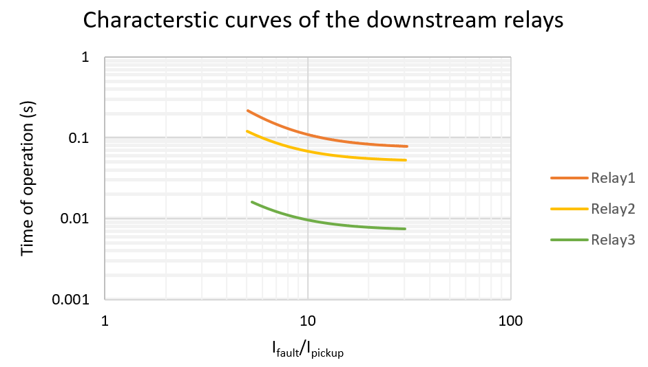
The characteristic curves of the downstream relays with the parameters from the table above are shown in the figure below:
* Fault studies were performed and the fault currents were noticed.
Coordination of the Upstream Relays
The upstream relay parameters are shown in the table below:
| Relay | Base Current (A) | Base Voltage (V) | 51P Pickup current (pu) | Time Dial (s) | Curve Type |
|---|---|---|---|---|---|
| 4 | 0.41 | 65.508 | 1.3 | 0.38 | U.S. Inverse (U2) |
| 5 | 0.09 | 65.508 | 2 | 0.305 | U.S. Inverse (U2) |
| 6 | 0.25 | 65.508 | 1.3 | 0.04 | U.S. Inverse (U2) |
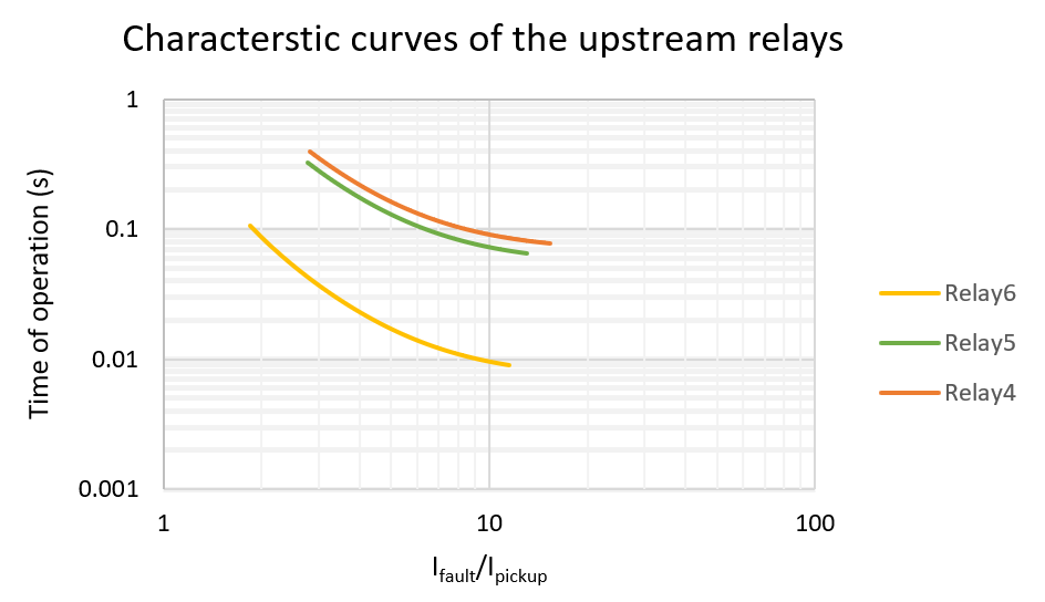
Characteristic curves of the upstream relays with the parameters from the table above are shown in the figure below:
Simulation and Results
To start the simulation in a steady-state, the network must be initialized by the Load Flow.
Open Network -> Load Flow and make sure the frequency is 60 Hz.
Open Simulation Settings and enable the option "Perform load flow and set initial conditions at simulation start". Make sure the time step is set to 50 us.
Warning: When executing in real-time on Redhat targets., model doesn't work with "opicc" in Settings – Target – Compiler and Linkerworks.
Case 1: Overcurrent coordination and the role of the backup protection scheme
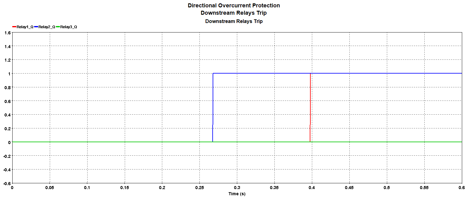
A three-phase-to-ground fault (ABC-G) is applied at t = 0.2 s on a 7 km lateral line connected at Bus 14 in section 2. Since the fault occurs in section 2, relays 2 and 5 should pick up and clear the fault by opening the Circuit Breaker (CB) 2 and 5 respectively.
It is demonstrated in this case that in the event of a breaker failure (example: CB 2 fails to operate), then relay 1, which is the backup protection for section 2 faults will pick up and clear the fault by opening CB 1. This demonstrates the coordination between overcurrent relays and the importance of backup protection. The test case is described in the figure below:
Steps to be followed:
Open the control panel of the line 'L8' which is a 7 km Lateral line connected at Bus 14 in section 2. Enable ‘Time programming’ in the ‘Timing’ tab.
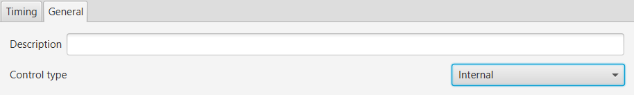
Open the control panel of Brk2, in the 'General’ tab, change the ‘Control type ’ from 'External (input pins)' to 'Internal' as follows:
This allows Brk2 to not to be controlled by relay 2 output. This is to simulate a breaker failure scenario.
Now, start the simulation and launch ScopeView, open the template: ‘Directional_Overcurrent.xml’.
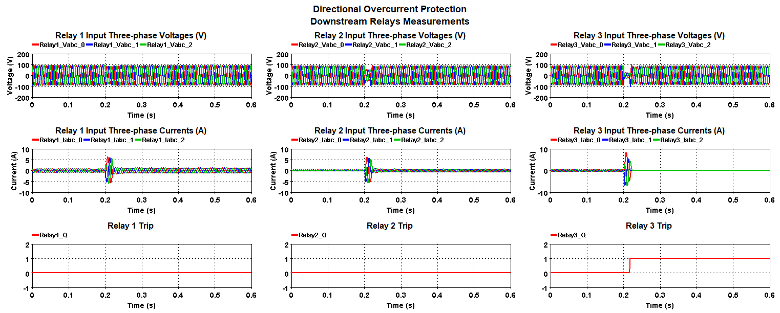
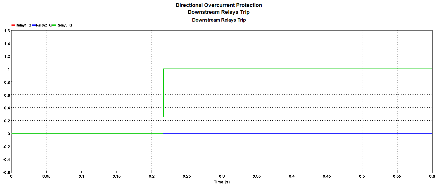
Make sure both ‘Sync’ and ‘Trig’ are checked, then start the data acquisition. The figure below shows the downstream relays voltages, currents, and the trip output.
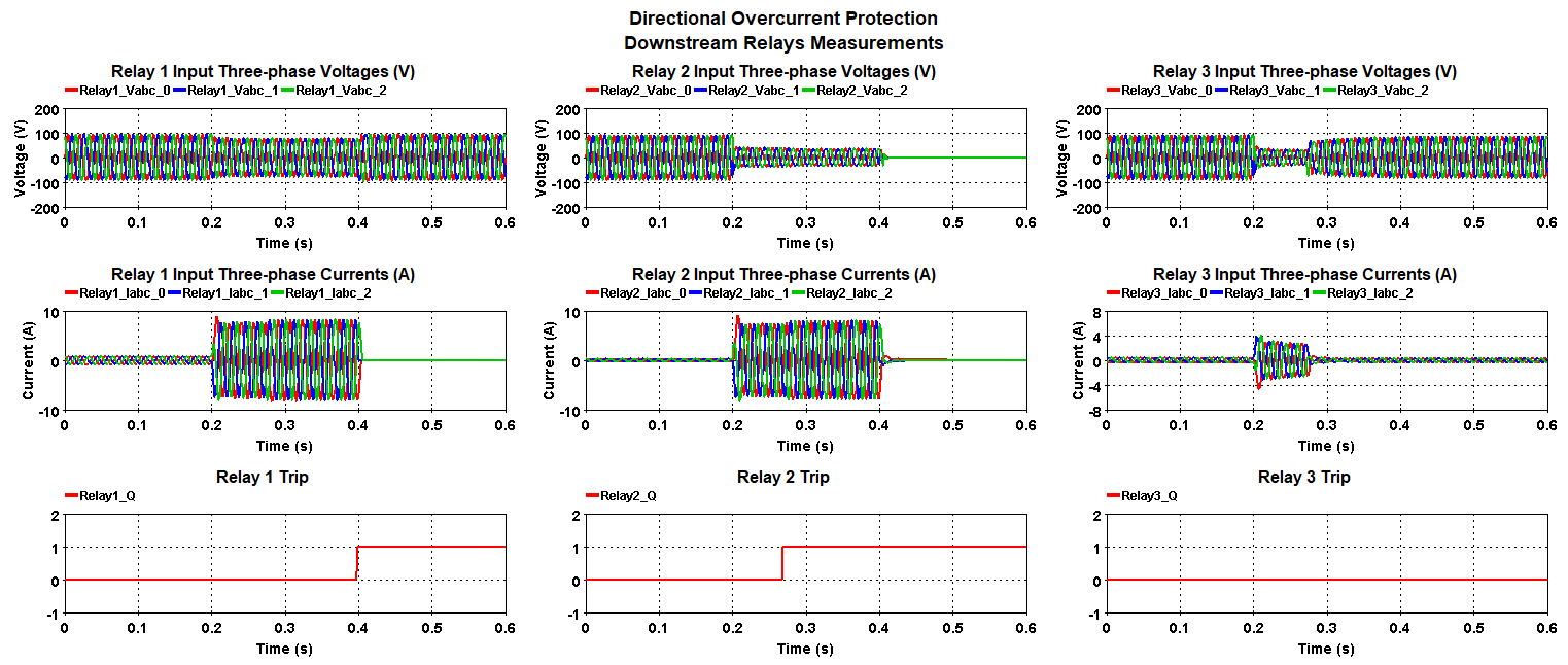
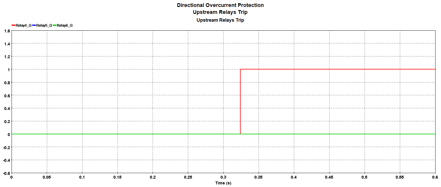
As shown in the figure below, the relay 2 picks up in 0.067 s (from the time of fault) and breaker 2 (supposed to be controlled by relay 2) fails to clear the fault. Relay 1 which is the backup protection for section 2 faults, picks up in 0.1975 s and clears the fault by opening breaker 1. This clearly demonstrates the coordination among the relays and the importance of a backup protection scheme.
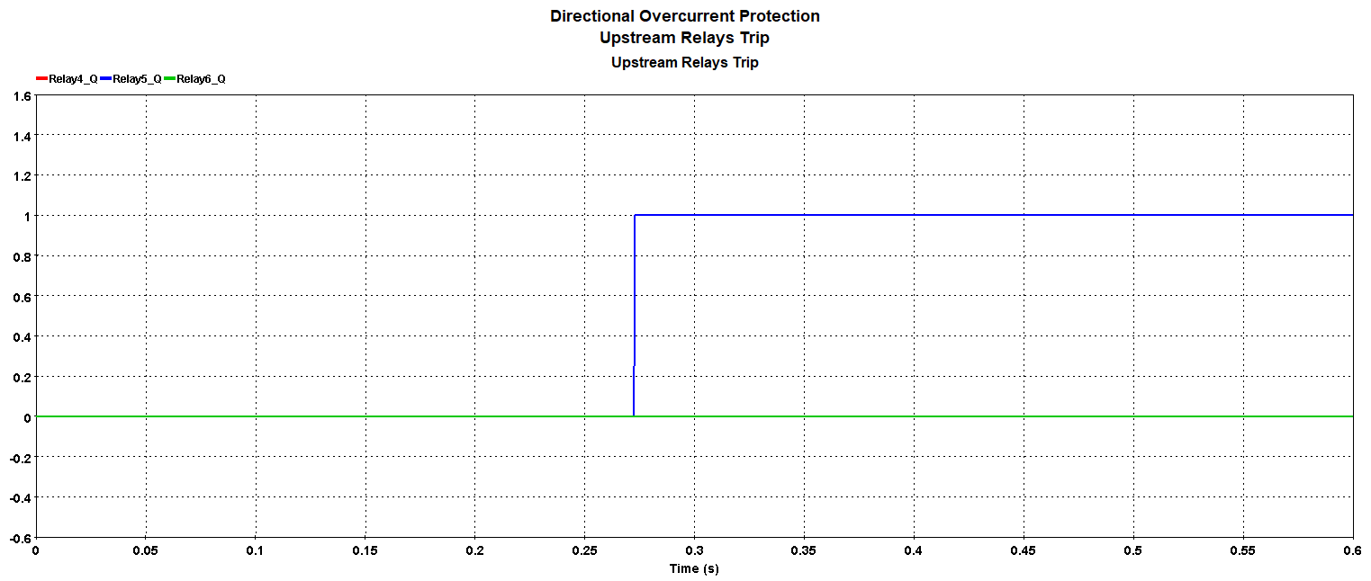
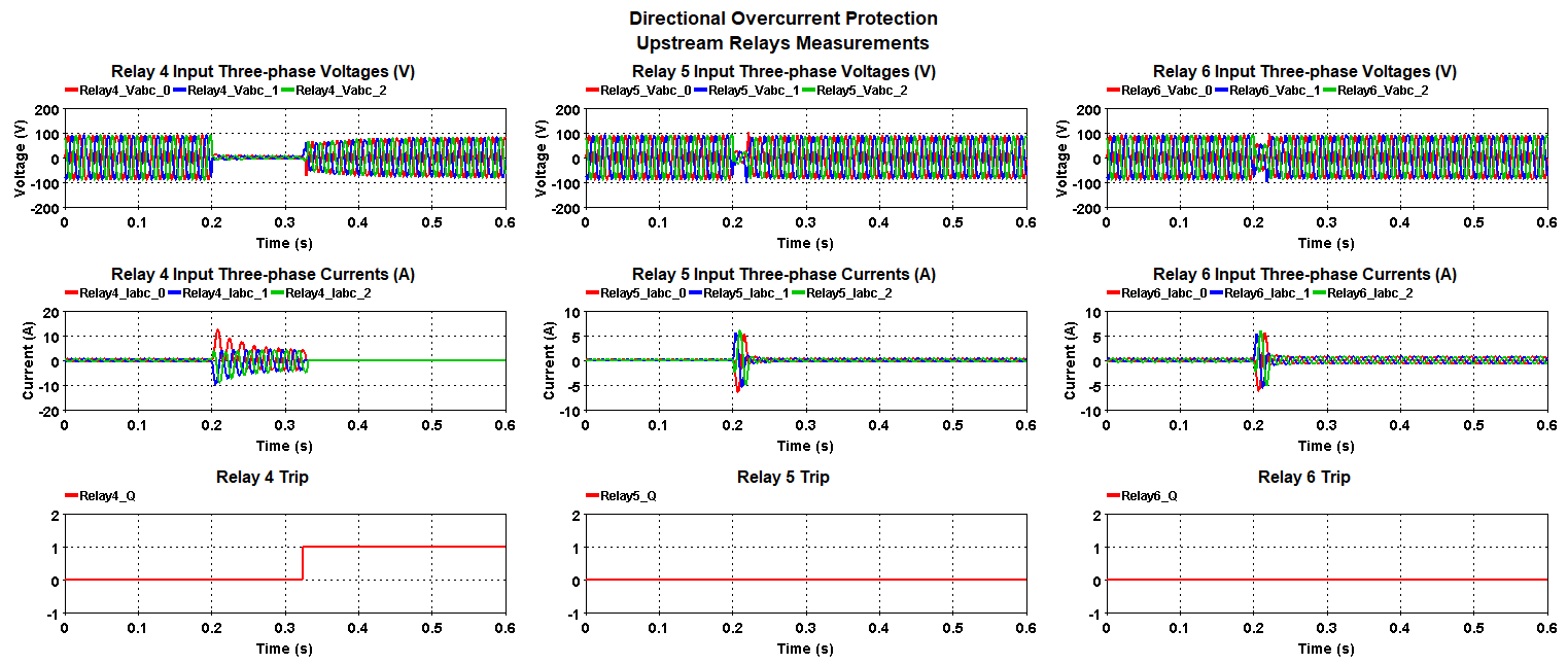
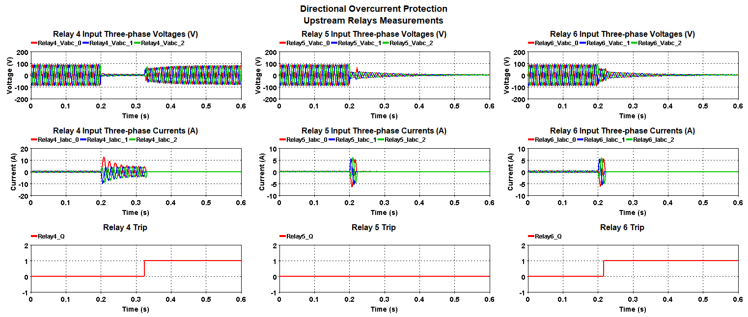
The figure below shows the upstream relays voltages, currents, and the trip output. Since the fault is in section 2 so relay 5 should pick up and clear the fault by opening CB 5.
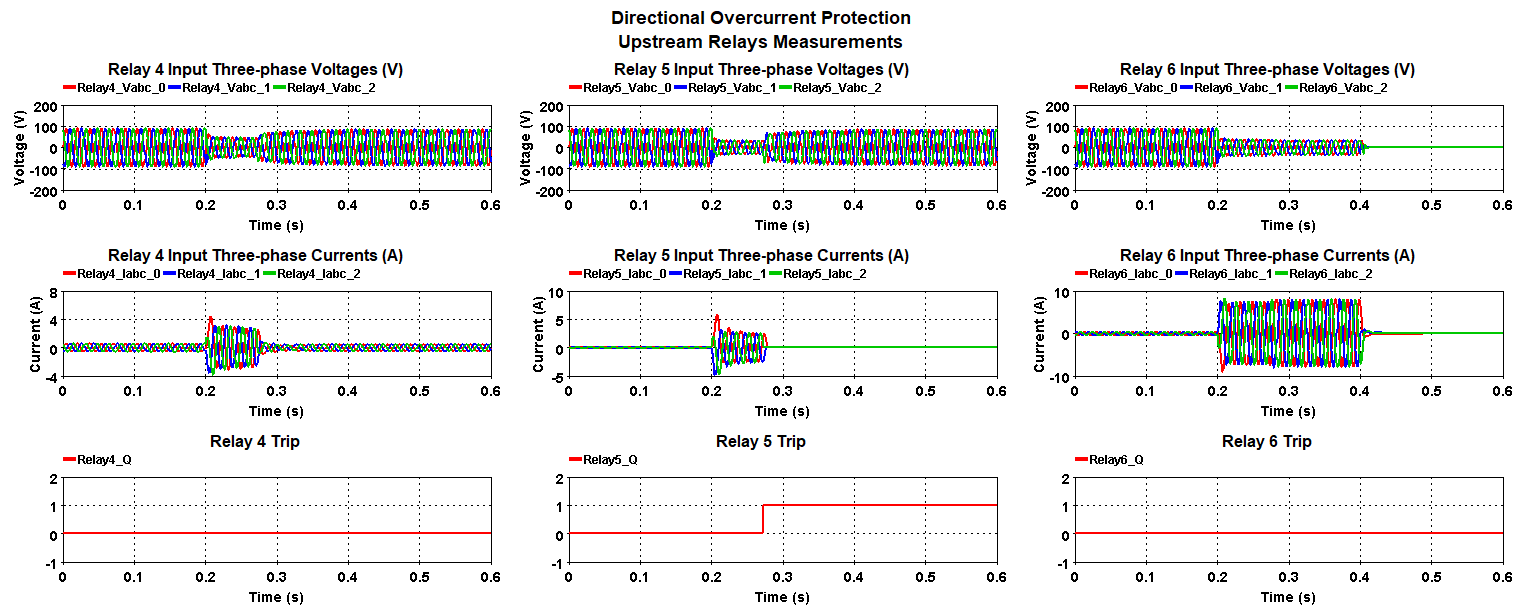
As shown in the figure below, relay 5 picks up in 0.0727 s (from the time of fault) and clears the fault by opening CB 5, as expected. Relay 4 and 6 do not operate.
Case 2: Importance of directional element in the protection scheme
A. When the directional element is enabled in the relays
A three-phase-to-ground fault (ABC-G) is applied at t = 0.2 s on a 6 km line connected between Bus 26 and 30 in section 3. Since the fault is applied in section 3, all the downstream relays (1,2 and 3) will see the fault direction in the set direction but relay 3 with the lowest Time Dial setting will pick up and clear the fault. The upstream relays 5 and 6 will see the fault direction opposite to the set direction therefore will not respond. The upstream relay 4 which is non-directional will pick up and clear the fault.
The test case is described in the figure below:
Steps to be followed:
Stop the Simulation and make sure that the 'Enable phase directional 67P' setting of the relay 2, 3, and 5 is checked.
Open the control panel of the line 'L8' which is a 7 km Lateral line connected at Bus 14 in section 2. Disable ‘Time programming’ in the ‘Timing’ tab.
Open the control panel of the line 'L6' which is a 6 km line connected between Bus 26 and 30 in section 3. Enable ‘Time programming’ in the ‘Timing’ tab.
Open the control panel of Brk2, in the ‘General’ tab, change the ‘Control type’ from 'Internal' to 'External (input pins)'.
Start the simulation and observe the results in ScopeView.
The figure below shows the downstream relays voltages, currents, and the trip output.
As the fault is in section 3, relay 3 picks up first in 0.0161 s (from the time of fault) and clears the fault by opening breaker 3 as expected.
The figure below shows the upstream relays voltages, currents, and the trip output.
As the fault is in section 3, relay 4 picks up first in 0.1237 s (from the time of fault) and clears the fault by opening breaker 4 as expected.
B. When the directional element is disabled in the relays
The response of the protection system when the directional element (67P) is disabled is shown in this case. The fault conditions are similar as described in Case 2A.
Steps to be followed:
Stop the simulation and disable the directional element by unchecking the 'Enable phase directional 67P' setting of the relay 2,3,5 and 6. Start the simulation and observe the results in ScopeView.
The figure below shows the downstream relays voltages, currents, and the trip outputs. As all the downstream relays observe the fault, relay 3 with the lowest Time Dial (0.04 s) setting will pick up first.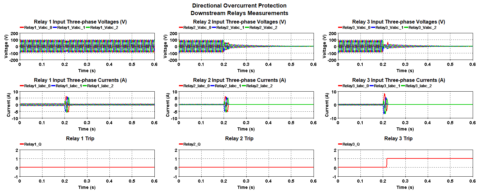
The figure below shows relay 3 picks up first in 0.0161 s (from the time of fault) and clears the fault by opening the breaker 3.

In upstream, relay 6 with the lowest Time Dial setting ( 0.04 s) will pick up first and isolate sections 2 and 3. The DG will still feed the fault as the fault is in section 3 so then relay 4 will pick up and clear the fault. The figure below shows the upstream relays voltages, currents, and the trip outputs.
It can be seen from the figure below that relay 6 (non-directional now) picks up in 0.0158 s (from the time of fault) and opens breaker 6. After CB 6 opens, the DG is still feeding the fault therefore relay 4 picks up in 0.1236 s (from the time of fault) and opens breaker 4 and clears the fault.
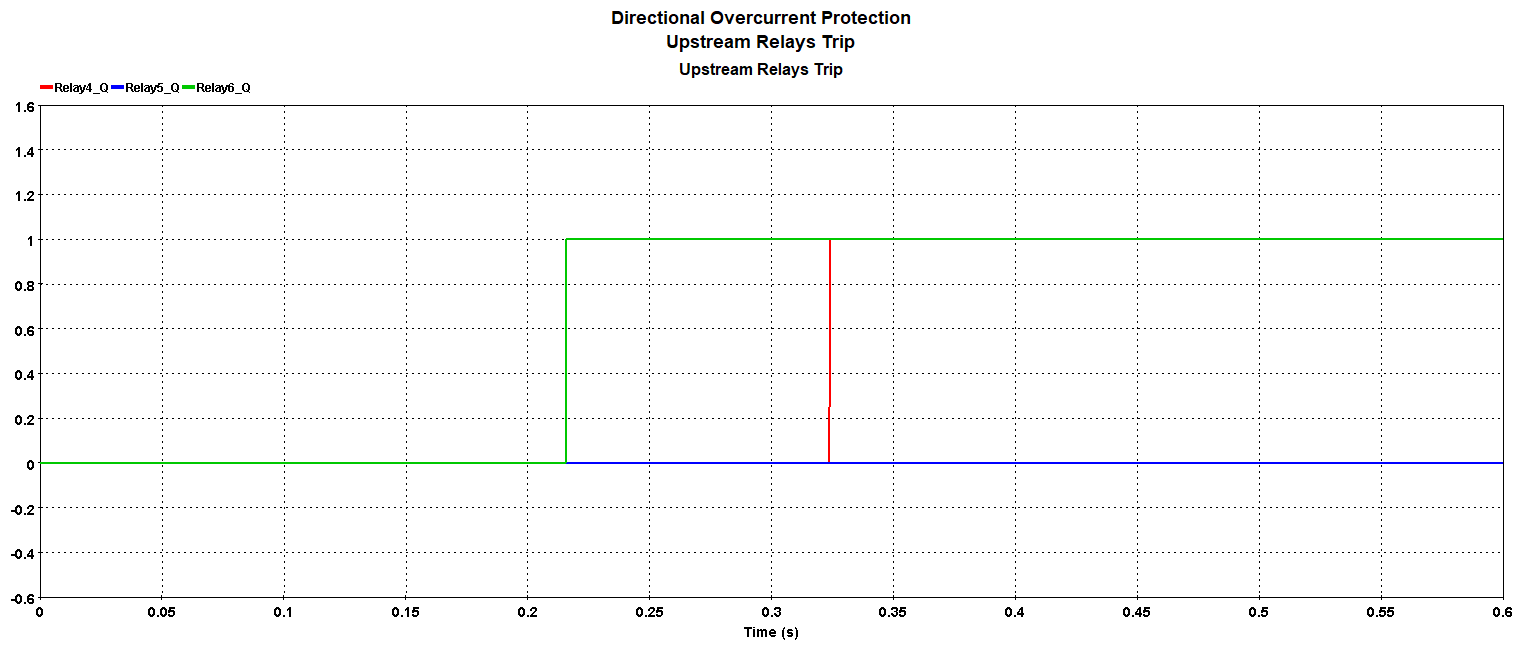
Note : It can be seen that even if relay 6 picked up in 0.0158 s (from the time of fault), relay 3 still observes the fault currents because of the breaker operation time delay. Relay 3 picks up in 0.0161 s (from the time of fault).
This shows that in the absence of directional elements the relays fail to discriminate between the healthy and faulty sections. This clearly demonstrates the importance of the directional element which provides selectivity to the Overcurrent relay.
OPAL-RT TECHNOLOGIES, Inc. | 1751, rue Richardson, bureau 1060 | Montréal, Québec Canada H3K 1G6 | opal-rt.com | +1 514-935-2323
Follow OPAL-RT: LinkedIn | Facebook | YouTube | X/Twitter