Documentation Home Page ◇ HYPERSIM Home Page
Pour la documentation en FRANÇAIS, utilisez l'outil de traduction de votre navigateur Chrome, Edge ou Safari. Voir un exemple.
Example 3: Using Excel to Define Input Parameters
See also: TestView - Quick Start
NOTE that the language of the .xls file should be considered. csv (comma-separated variable format) files rely on the comma to separate/import/export cells in Excel. In some languages and contexts, the period (.) and comma (,) are interchangeable.
Example 1 showed how to execute a test sequence that had only hardcoded values. Example 2 focused on the use of variables to define some parameters in the model. Example 3 will focus on the use of Excel to define the parameters of a test. This example will not go into much details regarding the blocks that were used in the first examples. It is recommended to do the two other examples before this one.
The starting point is the end of the Quick Start tutorial (Link to the Quick Start tutorial). Your TestView should now look like the Figure below.
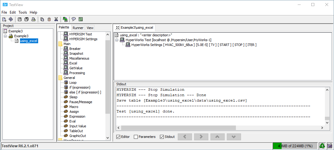
Starting Point: Example 3
This example will modify the resistance of Ld2 in the example HVAC_500kV_6Bus model and try different faults.
Similarly to example 1 and 2, let’s start by making sure that the options Start simulation and Disable Time Events are checked and unchecked, respectively in the HYPERSIM Settings block and let’s add a sleep of 1 second.
To make a complete example, add a 'take snapshot' command to the script before adding a loop (in auto-detect mode and operation option enabled). The script should now look like the Figure below.
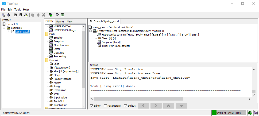
After adding the loop command
In the loop, it will be the execution section of the script. Therefore, we need to create the Excel file before going any further. Create a new Excel (xlsx) file anywhere. For this example, the Excel file was created inside the TestView project directory and named 'example3.xlsx'.
There are different ways to right the values of the parameters in the Excel file. Please consult this section for more information.
In the newly created file, fill it out like in the Figure below.
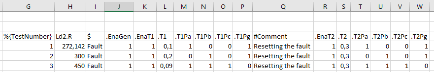
Quick Recap:
The name of the parameters can be found in the Netlist or by hovering the cursor over the parameter in the mask in HYPERSIM.
%{} defines variables that can be used exactly like the ones in example 2.
Ld2.R is a way to define the resistance of the load Ld2.
When several parameters inside the same component need to modified, it is possible to define them on several columns to lighten the lecture of the header. In the Figure above, the column 'I' (with the dollar sign) specifies the component and the following columns (starting by a period, followed by the name of the parameter) specify the values for the component 'Fault'.
In the Figure above, the first test will be an AG fault, the second test will be and BG fault and the third one, an ABC fault, all with different timings.
The # identifies a column that is a comment. It will not be taken into account by TestView when importing data.
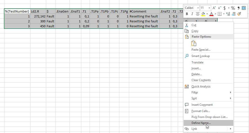
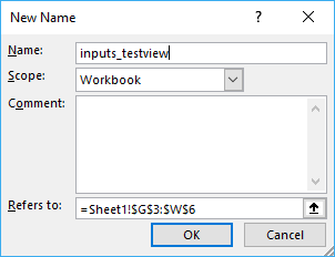
The next step is to define two named range: the first one is for the inputs and the second one is for the results. To define the input named range, select all the data (including the header), right-click and select 'Define Name...'. Any name can be given. In this example, we use 'inputs_testview'. Press OK.
Repeat the same steps, but with another range (that is empty) and define its name to 'output_testview'. This is were the results will be written by the 'TableOut' command. You do not need to select the exact size, TestView will automatically resize the range if the defined range is too small.
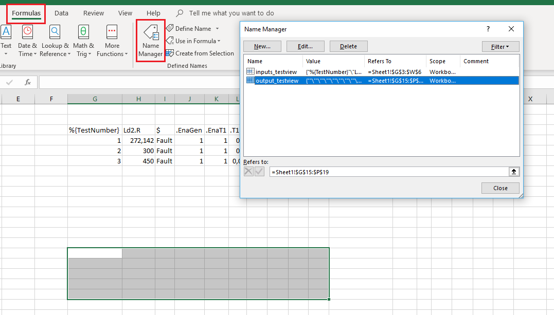
To verify that the named range were properly defined in Excel, go to the 'Formulas' ribbon and click on 'Name Manager'. Make sure the defined range are not overlapping. Save and close the Excel file.
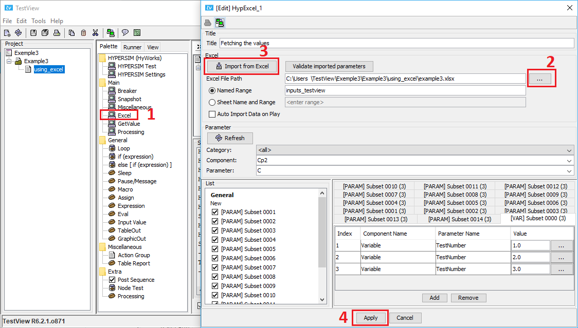
Back to TestView! Double click on the Excel command, click of the '...', select the Excel file that was created, press 'Import from Excel' and the data from Excel should appear in the parameter section, as presented below. Press Apply.
Add a snapshot command to load the snapshot taken previously. Add the same processing command as example 2 (fastest way is to copy-paste it from the previous example).
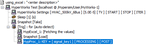
The test sequence should now look like the Figure below.
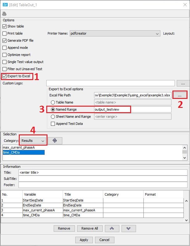
The last step is to add a TableOut command to export the results to Excel. To do so, double-click on 'TableOut' in the Palette tab. Select the 'Export to Excel' option, get the directory of the Excel file, change to 'named range' and type 'output_testview' and add the desired results. Press apply.
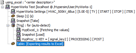
Be careful that the 'TableOut' block is not inside the the loop! The script should now look like:
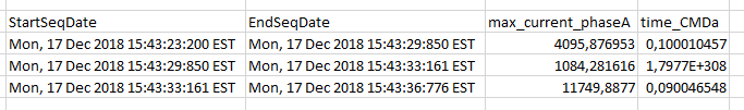
You can now run the test sequence. Once the test sequence is done, you can open the Excel file to see that the results were properly written:
Some closing notes
In the results, it is normal that 'time_CMDa' is 1.79e+308 because the second test is a BG fault. Phase A does not switch in this case.
The results can be written to a different Excel file, it does not need to be the same file.
Make sure that you re-import the data if you modify the Excel file or that the option 'auto-import on play' is checked. If not, the changes in the Excel file will not be seen by TestView.
By default, TestView will overwrite the same named range every time the test is re-run. There is an option called 'Append Test Data' in the 'TableOut' command to append the data instead of overwriting it. Be careful with the size of the file if this option is enabled.
OPAL-RT TECHNOLOGIES, Inc. | 1751, rue Richardson, bureau 1060 | Montréal, Québec Canada H3K 1G6 | opal-rt.com | +1 514-935-2323