Example 1: Changing the Timing of a Fault

This example starts from the Quick Start tutorial and adds blocks to control the timings of the fault in the HVAC_500kW_6Bus example model.

The test will iterate three times: the first time, the fault time will be 0.025s, the second time, it will be 0.050s and the third time it will be 0.075s. The changes are visible by looking at certain waveforms.

The starting point is the basic tutorial (only the names of the test, study and project is different in the screenshot below, the rest is identical to the basic tutorial). 

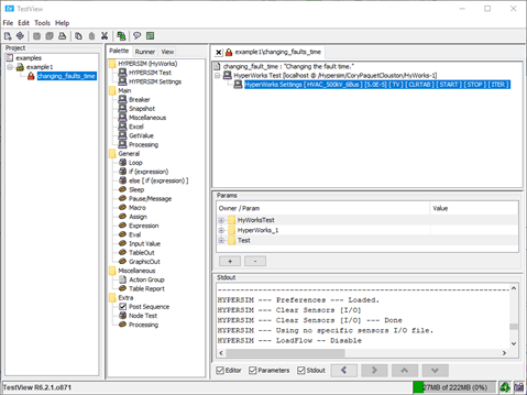
Starting Point of Example 1 (Same as Basic Tutorial)

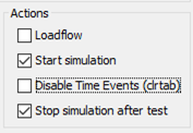
The first thing to do is to double click on the HyperWorks_1 block (the second block) and to validate that the option ‘Disable Time Events (clrtab) is unchecked.

Settings in HyperWorks (HYPERSIM Settings)

To continue, it is not mandatory but let’s add a one-second delay to make sure the simulation is in steady-state before applying the fault. To do so, go in the Palette tab and double-click on the ‘sleep’ block. The default value is one second. Therefore, simply press Apply. The script should now look like the figure below.

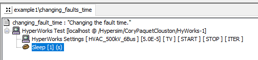
Test after Adding One Second Delay

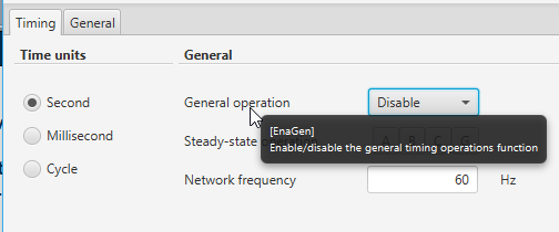
• If we go back to the model in HYPERSIM and double-click on the block named Fault, we can see that the General operation option is disabled (in the Timing tab).
• It could be manually enabled every time before running a test in TestView, or we could be sure it is enabled by forcing the value in the TestView Test.
• Make sure that T1 and T2 and Enabled and set for a phase A to G fault.
• Make sure that Steady-State Operation options are all grey (i.e. that there is no fault).
• These parameters could be set using TestView, but they are verified manually in this case.

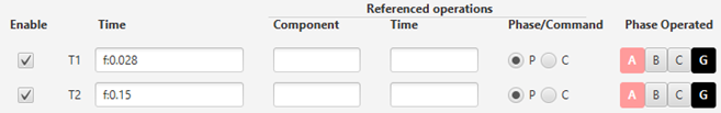
Switching Times T1 and T2 for Fault Block

Steady-State Operation of Fault Block

To enable it through TestView, it is necessary to find the name of the variable that represents this option. To do so, there are two options.

• The first option is tool tips/alt text: place the cursor over the field of the option, wait a second, and look for the name in brackets (see Figure 42, EnaGen in this case).
• The second option is to use the netlist in the HYPERSIM tab. In this window (see Figure 43), all blocks with all parameter names are present.

Fault Block in the HVAC_500kV_6Bus. EnaGen is the Name of the Option General Operation

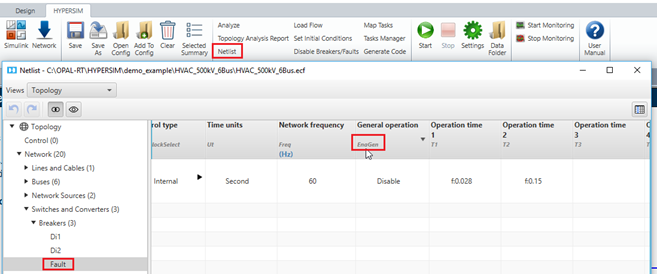
Netlist Window in HYPERSIM

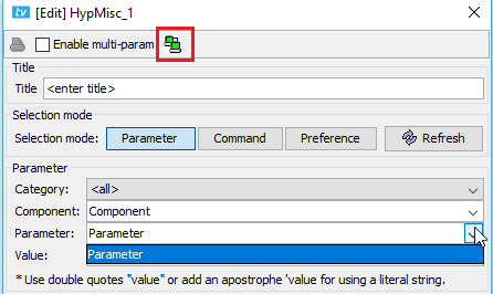
• Once the name of the parameter and its block to set are found, go back to TestView and add a new block called Miscellaneous.
• In this block, click the Parameter button.
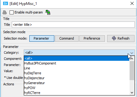
• If the drop-down menus do not have a list of all the blocks names and their parameters, the connection between the model and TestView is not working. It is most common HYPERSIM was closed on a TestView project without running the model again directly from HYPERSIM.
• There are various ways to force the reconnection: close TestView and HYPERSIM, open the copy of the model in the project directory ([Name of Project] \ bank \ hnk\ [Name of Project].ecf), run it and re-open TestView.
• Another approach is to open the Connection window (the computers in Figure 44), to disconnect and reconnect the model.

Miscellaneous Block. The Connection between the Model and TestView is not working (the dropdowns are empty).

Miscellaneous Block. The Connection between the Model and TestView is Working (the dropdowns menus are not empty)

Once the connection is correct, the component to select is the name of the block (i.e. Fault), the parameter (i.e. EnaGen), the value is 1 (to set to enable) and press add.

Users can add a description in the Title field to have a description visible in the Test Editor Window.

Press Apply to close the window and add the block to the script.

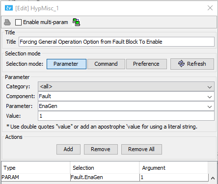
Forcing the General Operation of the Block Fault to Enable using the Miscellaneous Block

The block will not necessarily be added at the end of the script, it will be added below the selected block. If necessary, use one of the arrows to move the block in the Test (see Figure 47Figure 46 - also available by right-clicking on the block).

In the miscellaneous block, it is also possible to other options for the model, which are not in any blocks. For instance, it is possible to start or stop a simulation, enable load flow, etc. Those options are in the command mode (press the command button). The preference button is usually for lower-level types of calls, therefore it is usually less used.

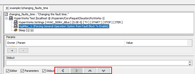
Arrows to Move a Block in a Test

Test after Adding Miscellaneous Block

• To summarize up to this point, the block HYPERSIM Settings sets the connection between the copy of the model and the test and starts the simulation. Afterwards, we wait one second to reach steady-state and we enable the fault breaker (meaning that it is ready to trig when asked to).
• To continue, the goal of this script is to repeat three times the same fault, but for different timings. Therefore, it will need a loop, but before that, let’s take a snapshot. The snapshot saves the currents and voltages (but not the states of the breakers, i.e. the type of faults for instance or if a breaker is enabled or not). This way, each of the tests will begin under the same conditions. In other words, the previous test will not affect the following test (for instance, if the system does not recover from a fault). Therefore, we do not need to stop and restart the simulation.
• Add a snapshot by double-clicking on Snapshot in the palette tab. Select the option ‘Take a snapshot of the simulation’ and press apply.

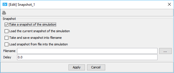
Setting the Snapshot Block to Take a Snapshot

To continue, the next block to add is the Loop. Select the option ‘User defined’ and the option ‘Operation’. Change the final value to 3 and press Apply.

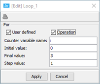
Setting the Loop Block to Iterate Three Times

In this case, each iteration of the loop represents one test (i.e. different fault time). Therefore, the first thing to do is to load the snapshot to make sure we are in the steady-state conditions before starting a new iteration.

Add a snapshot by double-clicking on Snapshot in the palette tab. Uncheck the option ‘Take a snapshot of the simulation’, check the option ‘Load the current snapshot of the simulation’ and press apply.

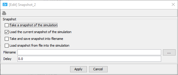
Loading a Snapshot

The next step is to define the different timings for the fault breaker. To do so, add a block named ‘Breaker’ by double-clicking on it, enable the option ‘multi-param’, select Fault in the Name dropdown, then, check SW_T1 and SW_T2. Press three times in the SW_T1 tab on the Add button and sets the different timings. The window should now look like Figure 52.

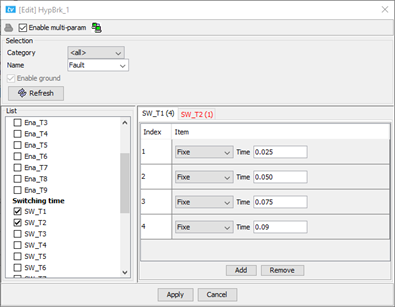
Breaker Block (Halfway Set – showing SW_T1 tab)

There are three points to notice at this point.

• The first is that there is the option ‘EnaGen’ in this block too, so it could have been another way to set it instead of using the Miscellaneous block (not visible in Figure 52 but it is one of the parameters in the list on the left).
• Second, the tab SW_T2 is in red. This is because that tab only has one row of values for that parameter whereas SW_T1 has four. If a parameter is added to this block, it must be defined as often as the the parameter that has the most rows.
• Third, the loop block defines the number of iterations. Since it is user-defined to three iterations, it will only do the three first row of the breaker block. Therefore, any value could be defined in the fourth row, it will not be executed. If you want the loop to do all the tests in the breaker blocks, then simply uncheck the option ‘user-defined’.

An unrelated example where it could be useful to check user-defined instead of unchecking it would be to re-do one specific test (say, the fourth test, then you would set the starting and final values accordingly).

Back to example, go to the SW_T2 tab and press three times on the ‘add’ button. The tab’s name should not be red anymore. Define the timings for each row.

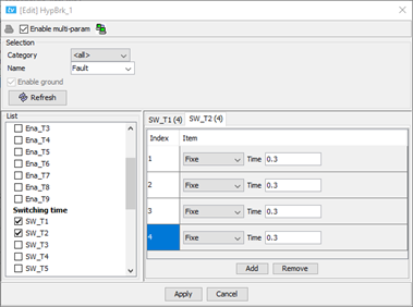
Breaker Block (All set - showing SW_T2 tab)

• Press Apply to close the window. The last block to add is the equivalent of pressing Play in ScopeView. It is the Processing block.
• Double-click on Processing in the Palette Tab in TestView to add it to the test. In the General tab, set the following options as shown (do not press Apply yet).
• Note that the sampling rate depends on the time-step defined in the model. The default value in the example model is 50us, therefore the sampling rate is 20000. The Synchronization option is equivalent to ‘Sync’ in ScopeView (it uses the POW block to synchronize the acquisition) and the Operation sequence Option is equivalent to ‘Trig’ in ScopeView (it trigs the events to occur, i.e. the fault and the line breakers in this case).

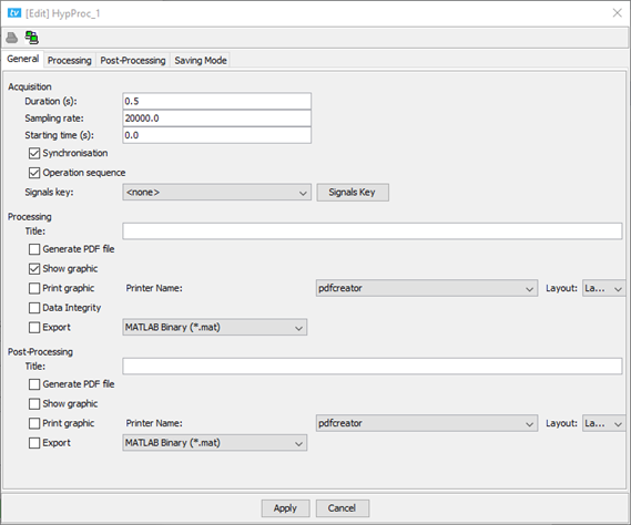
General Tab of Processing Block (Signals Key not yet Defined)

• The next step is to define the Signals Key. The Signal Key is equivalent to the Sensor Form in HYPERSIM. It is where you have access to all the signals from the model and where you select the relevant ones for analysis.
• Press the button ‘Signals Key’ in the Processing block and select the following signals (shown in Figure 55). The selected signals are the command signal from the Fault block (to validate that the timings are changing) and the currents from the breaker close to the Fault location.

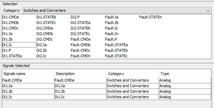
Signals Key

Press the save button and give a name to this new signal key. Press Apply to close the Signals Key window (to go back to the processing block).

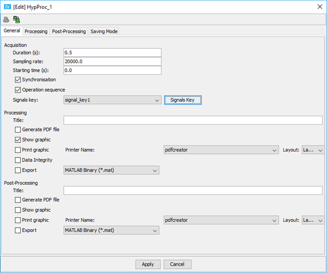
Processing Block (Signals Key Defined)

Once the Signals Key is defined, the next step is to define the signals to see after each test. To do so, go in the Processing tab (notice that the only signals available are the ones from the Signals Key) and add all those signals. This tab is the same as using ScopeView. After each test, a window will appear with those signals. Press Apply to close the window.

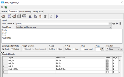
Setting the Signals in the Processing Tab of the Processing Block

The script should now look like Figure 58. The last step before executing the test is to select the option ‘Show’ in the Processing section of the View Tab.

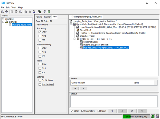
Complete Test for Example 1

To execute the test, select the option ‘Current Test Only’ in the Runner tab and press play (the arrow sign). The first window will appear, as shown in Figure 59. You need to close it before the next test runs. The second window will appear, close it, and so on until the end of the test.

A few points to note:

• In the Processing tab of the Processing block, you have access to all the ScopeView functions to do processing on the signals.
• Only three tests were run (even though four were defined) in the Breaker block. This is because the loop is hard-coded to do three iterations only. 
• To let TestView auto-detect the number of iterations to do, uncheck the ‘user-defined’ options in the Loop block.
• By default, the data is saved in COMTRADE format in the project directory. To have other format, there is the option ‘Export’ (visible in Figure 56) where you can select other types of format (in HYPERSIM 6.2+ only).
• To run a test without seeing the waveforms after each iteration, simply uncheck the option ‘Show’ in the View tab. This way, TestView will not wait between each test for the user to close a window.
• The fault is not exactly at 25ms because that number falls between two time-steps. It is not possible to have an event in between two time-steps. The fault occurs to the closest time-step of 25ms.
• The fault is cleared for about 100ms (i.e. only a green line visible in Figure 59) because the fault breaker Di1 is opening at 0.1 second and closes again at 0.2s. In this case, the reclosing does not make sense because the fault is not yet cleared (it clears at 0.3s). Since it is hardcoded, it should be changed to say, 0.35s.

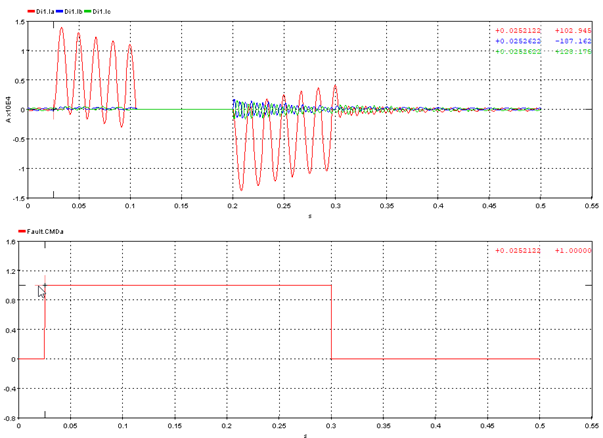
Results of the First Test (Currents where Superimposed)