Documentation Home Page ◇ HYPERSIM Home Page
Pour la documentation en FRANÇAIS, utilisez l'outil de traduction de votre navigateur Chrome, Edge ou Safari. Voir un exemple.
TestView Command | Main | Excel
- Sylvain Ménard

The Excel command offers an alternate way to define the parameters for the different iterations of a test. Instead of defining the values in the miscellaneous command or in the breaker command, it is possible to set everything in an Excel file which will be read by TestView using the Excel command. In other words, it allows the user to easily import parameters from Excel worksheets and copy them on the corresponding power system components when executing a series of tests.
Once the data has been imported, the list section and the component parameter sections are updated. After an import, it’s possible to add new components and parameters like in a multi-parameter miscellaneous command. The user simply has to select the name of the component, the parameter and then the option «New». A new tab for multiple parameters will be added. It will then be possible to add the number of required values. Each line corresponds to a value.
FIELD NAME | DESCRIPTION |
EXCEL WORKBOOK INFORMATION SECTION | |
Excel File Path | Path and name of the Excel file to use when importing parameter values. |
Named Range | Name of the Excel region where parameters are located in the Excel file. See section on Named region to get more information on how to define region names. Syntax Example : MyTable |
Sheet Name and Range | Excel range where parameters are located in the Excel File. The range must include the name of the sheet and all heading cells. Syntax Example : Sheet1!A1:G15 See section on Excel Range to get more information on how to define a sheet name and range. |
Import from Excel | By clicking this button, TestView will read the Excel file and import the parameters from the file. |
Auto Import Data on Play | When this option is checked, TestView will automatically import Excel data at the beginning of the test sequence. |
PARAMETERS SECTION | |
Category | Category of the component the user would like to select from if he wants to add new parameters. |
Component | Name of the component the user would like to add to the list. |
Parameter | Name of the component the user would like to add to the list. |
LIST SECTION | |
New | Add a new subset to the list of subsets. The new subset will use the component and parameter defined in the parameter section. |
Subset item | List of subset items used by TestView while iterating the loop. |
SUBSET SECTION | |
Index | Iteration number. |
Component Name | Component that will change during the iteration. |
Parameter Name | Parameter for which the value will change during the iteration. |
Value | New value for the iteration. |
Add | Add a new iteration to the list. |
Remove | Remove an iteration from the list. |
You can add any number of parameters, but they must all have the same number of values (shown in parenthesis in the tab). A tab turns red when it does not contain a sufficient number of parameters.
Excel test definition
The Excel Worksheet allows users to define parameters for power system components. These parameters will be used by the TestView “auto” loop step. This means that every iteration of an “auto” loop will use a different set of parameters. Many parameters from various components can be changed at the same time. The user must specify component and parameter names and then specify the set of values they would like to use in iterations.
Note that the user can enter parameter data using several formats (explained in the following sections). There are also two ways to specify the area where data is stored for reading an Excel file.
Data import options
Excel provides two different approaches to specify which part of the Excel file will be imported by TestView: named range and sheet area. Each alternative is explained in the following paragraphs.
NAMED RANGE
To specify data to be imported in TestView, named range is the suggested approach. It allows user to create meaningful short names that are easier to use in TestView. Each name refers to a part (an area) of the Excel document. The area contains data to be imported: parameter names are found in the first header row, and their values are found and on the subsequent lines.
To add a named range, follow the instruction below:
- In Excel, select the cell, range of cells, or nonadjacent selections to be named.
- Click the Name box at the left end of the formula bar.
![]()
- Type the name to use for the selection and then press Enter.
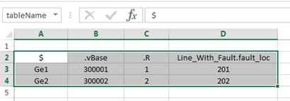
The following figure shows an example of named range. Its area is the range Sheet1:A2:D4
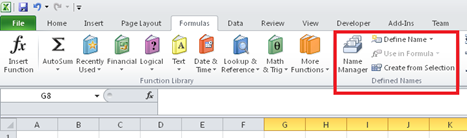
The Define Name toolbar can also be used to create new area in the Excel document. The following figure shows the Excel toolbar. See Excel help for more detail on this topic.
SHEET RANGE
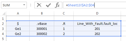
Alternatively, TestView can also import data by using a sheet range. No extra step is required in Excel to use this approach but the syntax is more complex to use in TestView since the user has to type the sheet range formula in TestView. The syntax for specifying a range is:
SheetName!$UpperLeftCell:$LowerRightCell
For example, a user that would like to read and import the table shown below will have to type Sheet13!$A$2:$D$4 in TestView step parameters.
Data Format Options
This section describes the various formats supported by TestView in the Excel file for defining which parameters to modify during tests. Each format offers different options: the first format allows only varying values of a single parameter for a single component during the test sequence and the other format allows users to vary the values of various parameters for a single component.
FIXED FORMAT
This format allows the user to define the values for one parameter while iterating a TestView loop. The component and the parameter are fixed for all iterations, but values are modified. The Figure below shows the generic definition of this format.
In this format, only one column is required. The header of the column specifies the component name and parameter name. Component and parameter names must be separated by a “.” symbols as in the following example: MyComponent.MyParameter. Following the header, subsequent rows will contain the iteration values.
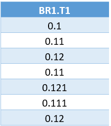
The Figure below shows an example for setting the operation time of the BR1 breaker. 7 iterations will be performed. T1 parameter will be set to 0.1 on the first iteration, 0.11 on the second iteration and so on.
VARIABLE COMPONENTS FORMAT
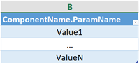
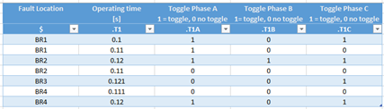
The second format allows the user to simultaneously set the values of various parameters for one component. For every iteration, the name of the component must be defined. It implies that the user can set many parameters for a component during some iterations but then switch to another component while iterating. The Figure below shows the generic definition of this format.
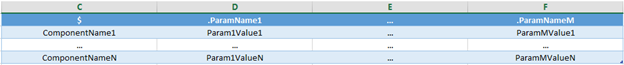
In this format, the first column specifies the component and the subsequent columns defines its parameters. The first column must be named “$”(column C in the Figure above) and the user must define the name of the component for each row. The subsequent columns must start with a period followed by the name of the parameter to update. Any number of parameters for one component can be defined.
The Figure below shows an example for operating various breakers. The operation time and the phase (A, B or C) to toggle are set at the same time. Again, in this example, 7 iterations will be performed. In the first iteration, the A, C and G phases of BR1 breaker are operated at 0.1 second, or toggled from their current state condition. In the second iteration, the same breaker is operated, but now, only phase A and G are toggled. Note that iterations 3 and 4 will then be performed on BR2 breaker. And so on.
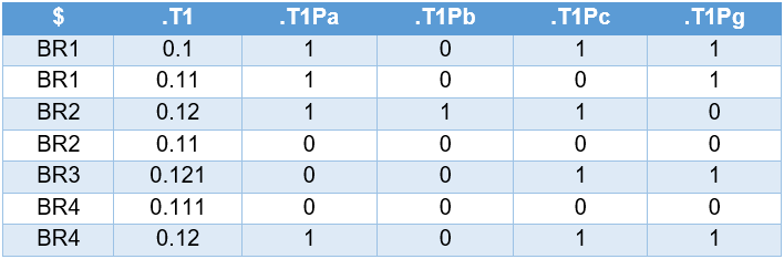
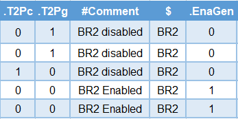
WARNING: The values of the parameters do not reset after each test! For instance, the second row (i.e. the second test) in the Figure above sets the breaker B1 with an AG fault. The third row (i.e. the third test), the AG fault on breaker BR1 is still enabled. Therefore, during the third test, BR1 AND BR2 will toggle their status.
In other words, it is important to make sure that the all the parameters are properly set. For that reason, it is recommended to have only one component per column. As an example:
COMBINING MULTIPLE FORMATS
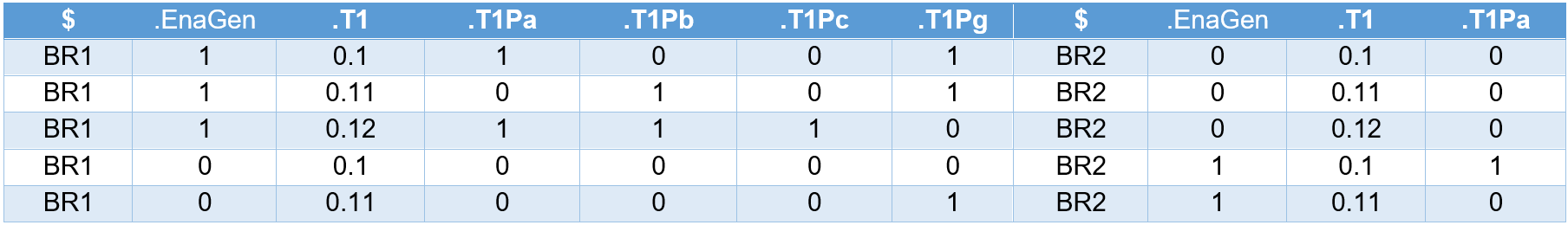
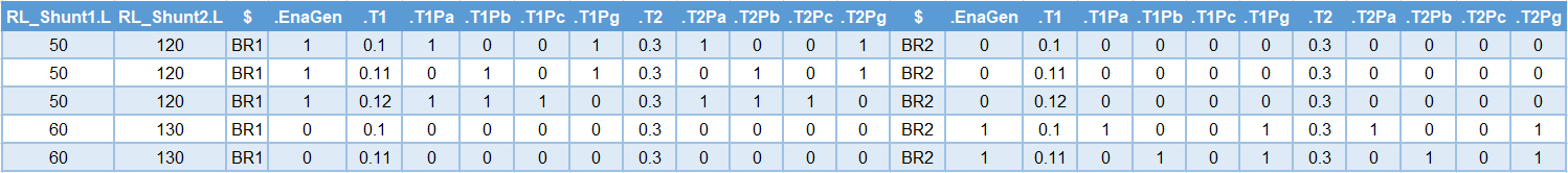
The user can combine and use both formats to control the changes of parameters for several components at the same time. The following figure presents one simple example where fixed format and variable components format are combined to set multiple parameters at the same time during loop iteration.
During the first iteration, the L inductance values are set on the RL_Shunt1 and RL_Shunt2 components to 50 and 120 MVAR respectively (note that there is no 106 factor because the units for this component is in MVAR). At the same time, operation time of the BR1 and BR2 breakers are set to 0.1 second and BR2 is disabled (EnaGen = 0). Therefore, the first iteration will execute an AG fault with BR1 that is cleared after 0.3 seconds. The second iteration performs very similar operations but with different values (BG fault at 0.11 second that is cleared after 0.3s).
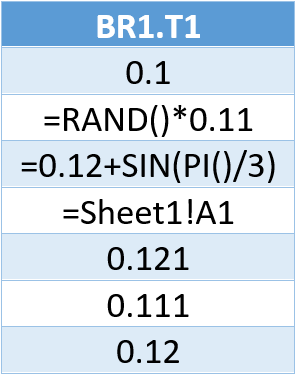
FORMULAS
Any cell of the table can contain standard Excel formulas. When TestView reads the Excel worksheet, values will be interpreted and only resulting numbers and text will be used. The following figure presents three cells where formulas are used to define the operating time of BR1 breaker. In the second iteration, the random function is used to generate a new number every time the worksheet is read. A uniformly distributed number between 0 and 0.11 is automatically generated. In the third iteration standard math functions are used. The fourth iteration uses a cell reference to cell A1 to define the operating time of the breaker.
EMPTY CELL
When the user leaves a cell empty, it indicates to the TestView sequencer to skip the change of the corresponding parameter value when iterating a loop. This can be useful when a change is not relevant for some iterations.
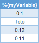
IMPORT VARIABLE
It’s possible to assign a value to a variable using Excel. In order to do this, the column header needs to use the syntax “%{myVariable}“. Variables can be used in TestView to change the execution sequence (ex: in If conditions) or in any step. Reminder: variables can be accessed in TestView steps with the following syntax: %{myVariable}.
ADD COMMENTS COLUMN
It’s possible to add a comments column in the Excel table. To do this, the header of the column must start with the “#” character. The # signifies that the column is completely ignored during the import process.
STYLE AND DESCRIPTIVE HEADERS
The user can apply any style and layout to tables without affecting data that will be imported in the TestView sequence. The user can also change cell content around the table.
OPAL-RT TECHNOLOGIES, Inc. | 1751, rue Richardson, bureau 1060 | Montréal, Québec Canada H3K 1G6 | opal-rt.com | +1 514-935-2323
Follow OPAL-RT: LinkedIn | Facebook | YouTube | X/Twitter